Chapter 5
Diffusion. Parabolic Partial Differential Equations
5.1 Diffusion Equations
The diffusion equation,
arises in heat conduction
, neutron
transport
, particle diffusion
, and
numerous other situations. There is a clear difference between the
time variable,
, and the spatial variables
. We'll talk
mostly for brevity as if there is only one spatial
dimension
, but this discussion can readily be generalized to
multiple spatial dimensions. The highest time derivative is
, first order. The highest spatial derivative is
second order
. The equation is classified as parabolic.
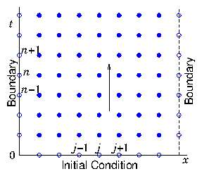
Figure 5.1: Solving a diffusion problem generally requires a
combination of spatial boundary conditions and temporal initial
condition. Then the solution is propagated upward (forward in
time), to fill in the multi-dimensional (time and space) solution
domain.
Consequently, boundary conditions
are not applied all around a closed contour (in the
-
plane) but
generally only at the two ends of the spatial range, and at one
"initial" time, as illustrated in Fig.
5.1. The
dependent variable solution is propagated from the initial condition
forward in time (conventionally drawn as the vertical direction).
5.2 Time Advance Choices and Stability
5.2.1 Forward Time, Centered Space
For simplicity we'll take
to be uniform in one cartesian
dimension, and the meshes to be uniform with spacing
and
. Then one way to write the equation in discrete finite
differences is
|
|
|
We use
to denote time index, and put it as a superscript to
distinguish it from the space indices
[
,
]. Of course this
notation is
not raising to a power. Notice
in this equation the
second order derivative in space is
naturally centered and symmetric. However, the time derivative is not
centered in time. It is really the value at
, not at the time
index of everything else:
. This scheme is therefore "Forward" in
Time, but Centered in Space (FTCS)
; see Fig.
5.2.
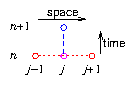
Figure 5.2: Forward Time, Centered Space, (FTCS) difference scheme.
We immediately know from our previous experience that, because it is
not centered in time, this scheme's accuracy is going to be only first
order
in
. Also, this scheme is
explicit in time. The
at
is
obtained using only prior (
) values of the other quantities:
|
|
|
A question then arises as to whether this scheme is
stable. For an ordinary
differential equation, we saw that with explicit integration, there
was a maximum step size that could be allowed before the scheme became
unstable. The same is true for hyperbolic and parabolic partial
differential equations. For stability analysis, we ignore the source
(because we are really analysing the deviation of the
solution
). However, even so, it's a bit
difficult to see immediately how to evaluate the amplification
factor
, because for partial differential
equations there is variation in the spatial dimension(s) that has to
be accounted for. It wasn't present for ordinary differential
equations. The way this is generally handled is to turn the partial
differential equation into an ordinary differential equation by
examining separately all the
Fourier
components of the spatial
variation. This sort of analysis is called Von Neumann
stability analysis. It gives a precisely correct
answer only for uniform grids and coefficients, but it is usually
approximately correct, and hence in practice very useful even for
non-uniform cases.
A Fourier component varies in space like
where
is
the wave number in the
-direction, (and
is here the square root
of minus 1). For such a Fourier component,
, so that
and
. Therefore
|
|
|
Then substituting into eq. (
5.3) for this Fourier
component we find
|
|
|
The amplification factor from each step to the next is the square
bracket term. If it has a magnitude greater than 1, then instability
will occur. If
is negative it will in fact be greater than
1. This instability is not a numerical instability, though. It is a
physical instability. The diffusion coefficient must be
positive otherwise the diffusion equation is unstable regardless of
numerical methods. So
must be positive; and so are
,
. Therefore numerical instability will arise if the
magnitude of the second
(negative) term in the amplification factor exceeds 2.
If
is small, then that will make the second term small
and unproblematic. We are most concerned about larger
values
that can make
approximately unity. In fact,
the largest
value that can be represented on a finite
grid
is such that the phase difference
(
) between adjacent values is
radians. That
corresponds to a solution that oscillates in sign between adjacent
nodes. For that Fourier component, therefore,
.
Stability requires
all Fourier modes to be stable, including
the worst mode that has
. Therefore the
condition for stability
is
There is, for the FTCS scheme, a maximum stable timestep equal to
.
Incidentally, the fact that
must therefore be no bigger
than something proportional to
makes the first order
accuracy in time less of a problem
. In
fact, for a timestep at the stability limit, as we decrease
, improving the spatial accuracy proportional to
because of the second order accuracy in space, we also improve the
temporal accuracy by the same factor, proportional to
because
.
5.2.2 Backward Time, Centered Space. Implicit Scheme.
In order to counteract the instability, we learned earlier that
implicit schemes are helpful. The natural
implicit time advance is simply to say that we use the values of the
updated variables to evaluate the rest of the equation, instead of the
prior values:
|
|
|
This is a Backward in Time, Centered in Space scheme; illustrated in
Fig.
5.3.
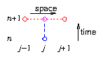
Figure 5.3: Backward time, centered space, (BTCS) difference scheme.
We'll see a little later how to actually solve this
equation for the values at
, but we can do the same stability
analysis on it without knowing. The combination for the spatial
Fourier mode is just as in eq. (
5.4), so the update
equation (ignoring
) for a Fourier mode is
|
|
|
The amplification factor is the inverse of the square bracket factor
on the left. That square bracket has magnitude always greater than
one. Therefore the BTCS
scheme is
unconditionally stable. We can take timesteps as large as we
like.
It turns out, however, that the only first order accuracy of this
scheme, like the FTCS scheme, means that we don't generally want much to
exceed the previously calculated stability limit. If we do so, we
increasingly sacrifice temporal accuracy, even though not stability.
5.2.3 Partially implicit, Crank-Nicholson schemes.
The best choice, for optimizing the efficiency of the numerical
solution of diffusive problems is to use a scheme that is part forward
and part backward. A combination of forward and backward, in which
is the weight of the implicit or backward proportion, is
to write
|
|
This is sometimes called the "
-implicit" scheme.
The amplification factor
is straightforwardly
|
|
|
If
then
, and the scheme is always
stable. If
, then
requires the
stability criterion
|
|
|
Thus the minimum degree of implicitness that guarantees
stability for all sizes of timestep is
. This
choice is called the "Crank-Nicholson" scheme.
It has a major advantage beyond stability. It is centered in
time. That means it is
second order
accurate in time (as well as space). This accuracy makes it useful to
take bigger steps than would be allowed by the (explicit advance)
stability limit.
5.3 Implicit Advancing Matrix Method
An implicit or partially implicit
scheme for
advancing a parabolic equation generally results in equations
containing more than one spatial point value at the updated time, for
example
,
,
. Such an equation for all spatial positions can
be written as a matrix equation. Gathering together the terms at
and at
from eq. (
5.9), it can be written
|
|
|
or symbolically
where
is the total length of the spatial mesh (the maximum of
), and the coefficients are
|
|
|
|
|
|
|
|
|
[Notice the
scaling factor in
.]
We are here assuming that the source terms do not depend upon
.
Eq. (
5.13) can be solved formally by inverting the matrix
:
|
|
|
Therefore the additional work involved in using an implicit scheme is
that we have (effectively) to invert the
matrix
, and multiply by the inverse at each timestep.
Provided the mesh is not too large, this can be a managable
approach. In a situation where
and
do not change
with time, the inversion
need only be done once; and each step in time
involves only a matrix multiplication by
of the
values from the previous timestep,
.
If the matrix has the tridiagonal
form of eq. (
5.12), where the entries are non-zero only on the
diagonal and the immediately adjacent subdiagonals, then it will
certainly be more computationally efficient to solve for the
updated variable by elimination
rather than inverting the matrix
and multiplying. This is a reflection of the fact that the matrix
is
sparse. All but a very small
fraction of its coefficients are zero. The fundamental problem is that
the inverse of a sparse matrix is generally not sparse. Consequently,
even though multiplication by the original sparse matrix actually
requires only a few individual arithmetic operations, and easy
short-cuts can be implemented, there are no obvious short-cuts for
doing the matrix multiplication by the inverse. As long as we are
implementing solutions in a mathematical system like
Octave
using the built-in facilities, we won't notice
any difference because we are not using short-cuts.
5.4 Multiple Space Dimensions
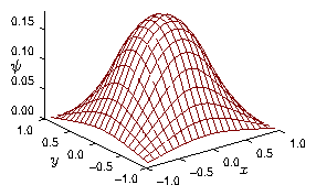
Figure 5.4: Example solution, at a particular time, of a diffusion
equation in two space dimensions. The value of
is
visualized in this perspective plot as the height of the
surface.
When there is more than one spatial coordinate dimension, as
illustrated in Fig.
5.4, nothing
changes formally about our method of solution of parabolic equations.
What changes, however, is that we need a systematic way to turn the
entire spatial mesh in multiple
dimensions
into a column vector like
those in eq. (
5.12). In other words, we must index
all the spatial positions with a single index
. But generally if we
have multiple dimensions, the natural (physical) indexing of the
elements of the mesh is by a number of multiple indices equal to the
number of dimensions: e.g.
, where
,
,
correspond to the coordinates
,
,
.
Reordering
the mesh elements is not
a particularly difficult task algebraically, but it requires an
intuitively tricky geometrical mental shift. In general, if we have a
quantity
indexed on a multidimensional mesh whose
lengths in the different mesh dimensions are
,
, ... then we
re-index them into a single index
as follows. Start with all
indices equal to 1. Count through the first index,
. Then
increment the second index
and repeat
. Continue this
process for
. Then increment the next index (if any), and
continue till all indices are exhausted. Incidentally, this is
precisely the order in which the elements
are
stored in computer memory
when using a
language like Fortran
when using the entire
allocated array.
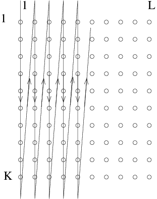
Figure 5.5: Conversion of a two-dimensional array into a single column
vector using column order is like stacking all the columns below
one another.
The result is that for the giant column vector
, the first
elements are the original multidimensionally indexed elements
; the next
elements,
,
are the original
and so on.
In multiple dimensions, the second derivative operator (something like
) is represented by a stencil
, as illustrated
in eq. (
4.23). The importance of the reordering of the
elements into a column vector is that although the components of the
stencil that are adjacent in the first index (
) remain adjacent in
, those in the other index(es) (
) do not. For example the
elements
and
have
-indices
and
respectively; they are a distance
apart. This fact means that for multiple spatial dimensions the
matrices
and
are no longer simply
tridiagonal. Instead, they have an additional non-zero diagonal, a
distance
from the main diagonal. If the boundary conditions are
, each matrix is
"Block-Tridiagonal"
,
having a form like this:
|
|
|
Here,
denotes the coefficient of the
center of the stencil,
and
denotes the coefficients of the
adjacent points in the
stencil. One can think of the total matrix as being composed of
blocks, each of size
. All the blocks are zero
except the tridiagonal ones. And each non-zero block is itself
tridiagonal (or diagonal). If there are further dimensions
, then
the giant matrix is a tridiagonal composite of
blocks,
each of a two dimensional (
block) type of eq. (
5.18). And so on.
It is very important to think carefully about the boundary
conditions
. These occur at the boundaries of
each block. Notice
how the corner (boundary) entries of the extra subdiagonal blocks make
zero certain coefficients of the subdiagonals of the total matrix.
One important consequence of the block-tridiagonal form
(
5.18) is that it is not so easy to do tridiagonal
elimination
rather than matrix inversion.
5.5 Estimating Computational Cost
The computational cost
of
executing different numerical algorithms often has to be considered
for large scale computing. This cost is generally expressed in the
number of floating point operations (FLOPs)
. Roughly, this is the
number of multiplications (or divisions) required. Additions are cheap.
For an
matrix, multiplying into a length-
column vector
costs (simplemindedly)
rows times
operations per row:
(FLOPs). By extending this to
columns, we see that multiplying two
matrices costs
. Although the process of
inversion of
a non-singular matrix, seems far more difficult to do, because the
algorithm is much more complicated, it also costs roughly
operations
. These estimates are accurate only
to within a factor of two or so. But that is enough for most purposes.
Inverting or multiplying random matrices using Octave on my laptop,
for
takes about 1 second. That seems amazingly fast to me,
because it corresponds to about 1 FLOP per nanosecond. But that's
about what can be achieved these days provided the cache contains
enough of the data.
Trouble is that if we are dealing with two-dimensions in space, each
of length
, then the side of the matrix we have to invert is
. A multiplication or inversion would take at least
seconds; that's a quarter of an hour. Waiting that
long is frustrating, and if many inversions are needed, time rapidly
runs out.
Inverting the matrix representing a two-dimensional problem takes
operations. And for a three-dimensional problem it's
.
This rapid escalation of the cost means that one doesn't generally
approach multidimensional problems in terms of simplistic matrix
inversion. In particular, it is difficult to implement an implicit
scheme for advancing the diffusion equation. And it is probably more
realistic just to use an explicit scheme, recognizing and observing
the stability
limit, eq. (
5.6), on maximum time-step size.
Worked Example: Crank Nicholson Matrices
Express the following parabolic partial differential equation
in two space variables (
and
) and one time variable (
)
as a matrix equation using the Crank-Nicholson scheme on uniform
grids.
|
|
|
Find the coefficients and layout of the required matrices if the boundary
conditions are
at
,
at
, and periodicity in
.
Let
and
be indices in the
and
coordinates, and let
and
denote their grid spacings. The
finite difference form of the spatial derivative terms is
|
|
Therefore, expressing the positions across the spatial grid in terms
of a single index
(where
is the size of the
-grid, and
of the
-grid), the differential operator
becomes a matrix
multiplying the vector
, of the form
|
|
|
The explanation of this form is as follows.
The coefficients of a generic row corresponding to
-position index
are
|
|
|
The periodic boundary
conditions
in
are implemented by the
appearance of off-diagonal,
-type, blocks at the upper right and
lower left of the matrix. The
-boundary conditions are the same for
all the blocks on the diagonal, the tridiagonal
-type blocks. At
the
boundary, (which would be the bottom row of each block), the
condition
means no contribution arises to the differential
operator from the
-value there. The condition therefore allows
us simply to omit the
row from the matrix, choosing the
index to refer to the position
. At the
end (the
top row of each block), the condition
can be implemented in a properly centered way by choosing the
-grid to be aligned to the half-integral positions.
In other words,
,
,
. (The
position values are not represented in the matrices.) In that
case, there is zero contribution to the difference scheme from the
first derivative at position
(because
there is
zero), and the
-second-derivative operator at
becomes
, giving rise to equal and
opposite coefficients
. The diagonal entry on those
rows is minus the sum of all the other coefficients on the row:
.
The Crank-Nicholson scheme for the differential equation time advance is then
|
|
|
which on rearrangement becomes
|
|
|
Exercise 5. Diffusion and Parabolic Equations.
1. Write a computer code to solve the diffusive equation
For constant, uniform diffusivity
and constant
specified source
. Use a uniform
-mesh with
nodes.
Consider boundary conditions to be
fixed, equal to
,
at the domain boundaries,
, and the initial condition
to be
at
.
Construct a matrix
such that
. Use it to implement the FTCS scheme
|
|
paying special attention to the boundary conditions.
Solve the time-dependent problem for
,
,
,
,
, storing your results in a matrix
, and
plotting that matrix at the end of the solution, for examination.
Experiment with various
to establish the dependence of the
accuracy and stability of your solution on
. In particular,
without finding an "exact" solution of the equation by any
other method,
(i) Find experimentally the value of
above which the scheme
becomes unstable.
(ii) Estimate experimentally the fractional error arising from finite
time step duration in
when using a
approximately equal to the maximum stable value.
(iii) By varying
, estimate experimentally the fractional error
at
arising from finite spatial differences. Which is more
significant, time or space difference error?
2. Develop a modified version of your code to implement the
-implicit scheme:
|
|
in the form
|
|
(i) Experiment with different
and
values, for the same
time-dependent problem and find experimentally the value of
for which instability disappears for all
.
(ii) Suppose we are limited to only 50 timesteps to solve over the time
so
. Find experimentally the optimum value
of
which produces the most accurate results.
Submit the following as your solution for each part:
- Your code in a computer format that is capable of being
executed, citing the language it is written in.
- The requested experimental and/or values.
- A plot of your solution for at least one of the cases.
- A brief description of how you determined the accuracy of the result.