Chapter 1
Introduction
1.1 What is a Plasma?
1.1.1 An ionized gas
A plasma is a gas in which an important fraction of the atoms is
ionized, so that the electrons and ions are separately free.
When does this ionization occur? When the temperature is hot enough.
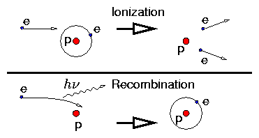
Balance between collisional ionization and recombination:
Figure 1.1: Ionization and Recombination
Ionization has a threshold energy. Recombination has not but is much
less probable.
Threshold is ionization energy (13.6eV, H) written
χi
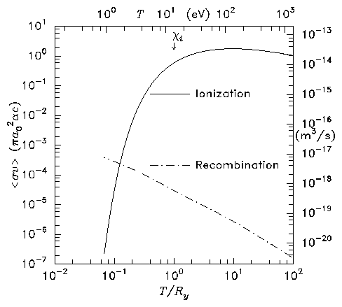
Figure 1.2: Ionization and radiative
recombination rate coefficients for atomic hydrogen
Integral over Maxwellian distribution gives rate coefficients
(reaction rates). Because of the tail of the Maxwellian
distribution, the ionization rate extends below T = χi.
And in equilibrium, when
|
|
nions
nneutrals
|
= |
< σi v >
< σr v >
|
, |
| (1.1) |
the percentage of ions is large ( ∼ 100%) if electron temperature:
Te >~χi/10.
e.g. Hydrogen is ionized for Te >~1eV
(11,600°K).
At room temperature ionization is negligible.
For dissociation and ionization balance figure see e.g. Delcroix
Plasma Physics Wiley (1965) figure 1A.5, page 25.
1.1.2 Plasmas are Quasi-Neutral
If a gas of electrons and ions (singly charged) has unequal numbers,
there will be a net charge density, ρ.
|
ρ = ne(−e) + ni(+e) = e (ni − ne) |
| (1.2) |
This will give rise to an electric field via
|
∇ . E= |
ρ
ϵ0
|
= |
e
ϵ0
|
(ni − ne) |
| (1.3) |
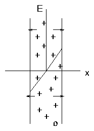
Example: Slab.
Figure 1.3: Charged slab
This results in a force on the charges tending to expel whichever
species is in excess. That is, if ni > ne, the E field
causes ni to decrease, ne to increase tending to reduce the
charge.
This restoring force is enormous!
Example
Consider Te = 1eV, ne = 1019m−3 (a modest plasma;
c.f. density of atmosphere nmolecules ∼ 3 ×1025m−3). Suppose there is a small difference in
ion and electron densities ∆n = (ni − ne)
Then the force per unit volume at distance x is
|
Fe = ρE = ρ2 |
x
ϵ0
|
= (∆n e)2 |
x
ϵ0
|
|
| (1.7) |
Take ∆n / ne = 1% , x = 0.10 m.
|
Fe = (1017 ×1.6 ×10−19)2 0.1 / 8.8 ×10−12 = 3 ×10⁶ N.m−3 |
| (1.8) |
Compare with this the pressure force per unit volume
∼ p/x with p ∼ ne Te (+ ni Ti)
|
Fp ∼ 1019 ×1.6 ×10−19 / 0.1 = 16 Nm−3 |
| (1.9) |
Electrostatic force >> Kinetic Pressure Force.
This is one aspect of the fact that, because of being ionized,
plasmas exhibit all sorts of collective behavior, different
from neutral gases, mediated by the long distance electromagnetic
forces E, B.
Another example (related) is that of longitudinal waves.
In a normal gas, sound waves are propagated via the intermolecular
action of collisions. In a plasma, waves can propagate when
collisions are negligible because of the coulomb interaction of
the particles.
1.2 Plasma Shielding
1.2.1 Elementary Derivation of the Boltzmann Distribution
Basic principle of Statistical Mechanics:
Thermal Equilibrium ↔ Most Probable State
i.e.
State with largest number of possible arrangements of micro-states.
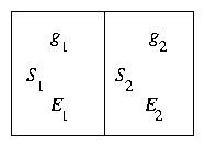
Figure 1.4: Statistical Systems in Thermal Contact
Consider two weakly coupled systems S1, S2 with energies
E1, E2. Let g1, g2 be the number of microscopic
states which give rise to these energies, for each system.
Then the total number of micro-states of the combined
system assuming states are independent is
If the total energy of combined system is fixed E1 + E2 = Et
then this can be written as a function of E1:
The most probable state is that for which [dg/(dE1)] = 0
i.e.
|
|
1
g1
|
|
dg1
dE
|
= |
1
g2
|
|
d g2
dE
|
or |
d
dE
|
lng1 = |
d
dE
|
lng2 |
| (1.13) |
Thus, in equilibrium, states in thermal contact have equal
values of [d/dE] lng.
One defines σ ≡ lng as the Entropy.
And [ [d/dE] lng ]−1 = T the Temperature.
Now suppose that we want to know the relative probability of
2 micro-states of system 1 in equilibrium. There are, in all,
g1 of these states, for each specific E1 but we want to know how
many states of the combined system correspond to a
single microstate of S1.
Obviously that is just equal to the number of states of system 2.
So, denoting the two values of the energies of S1 for the two
microstates we are comparing by EA, EB the ratio of the number
of combined system states for S1A and S1B is
|
|
g2 (Et − EA)
g2 (Et − EB)
|
= exp[ σ(Et − EA) − σ(Et − EB) ] |
| (1.14) |
Now we suppose that system S2 is large compared with S1 so that
EA and EB represent very small changes in S2's energy,
and we can Taylor expand the entropy of S2 (i.e. σ)
|
|
g2 (Et − EA)
g2 (Et − EB)
|
≅ exp | ⎡
⎣
|
− EA |
dσ
dE
|
+ EB |
d σ
dE
| ⎤
⎦
|
|
| (1.15) |
Thus we have shown that the ratio of the probability of a system
(S1)
being in any two micro-states A, B is simply
when in equilibrium with a (large) thermal "reservoir".
This is the well-known "Boltzmann factor".
You may notice that Boltzmann's constant (kB) is absent from this
formula. That is because of using natural thermodynamic units
for entropy (dimensionless) and temperature (energy).
Boltzmann's constant is simply a conversion factor between
the natural units of temperature (energy, e.g. Joules)
and (e.g.) degrees Kelvin. Kelvins are based on °C
which arbitrarily choose melting and boiling points of water and
divide into 100 intervals. Temperature in Joules = kB×
temperature in Kelvins.
Plasma physics is done almost always using energy units for
temperature. Because Joules are very large, usually electron-volts
(eV) are used.
|
1 eV = 11600 K = 1.6 ×10⁻¹⁹ Joules. |
| (1.17) |
One consequence of our Boltzmann factor is that a gas of moving
particles whose energy is 1/2 mv2 adopts the
Maxwell-Boltzmann (Maxwellian) distribution of velocities ∝ exp[ − [(mv2)/2T] ].
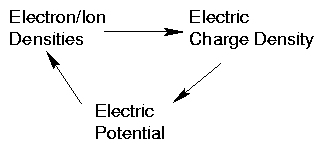
1.2.2 Plasma Density in Electrostatic Potential
When there is a varying potential, ϕ, the densities of electrons
(and ions) is affected by it.
If electrons are in thermal equilibrium, they will adopt a Boltzmann
distribution of density
This is because each electron, regardless of velocity possesses a
potential energy −eϕ.
Consequence is that (fig 1.5)
Figure 1.5: Self-consistent loop of dependencies
a self-consistent loop of dependencies occurs.
This is one elementary example of the general principle of plasmas
requiring a self-consistent solution of Maxwell's equations of
electrodynamics plus the particle dynamics of the plasma.
1.2.3 Debye Shielding
A slightly different approach to discussing quasi-neutrality leads to
the important quantity called the Debye Length.
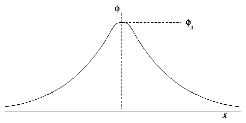
Figure 1.6: Shielding of fields from a 1-D grid.
Suppose we put a plane grid into a plasma, held at a certain
potential, ϕg.
Then, unlike the vacuum case, the perturbation to the potential falls
off rather rapidly into the plasma. We can show this as follows.
The important equations are:
| |
|
|
∇2 ϕ = |
d2ϕ
dx2
|
= − |
e
ϵ0
|
(ni − ne) |
| | (1.19) |
| |
|
| | (1.20) |
|
[This is a Boltzmann factor; it assumes that electrons are in thermal
equilibrium. n∞ is density far from the grid (where we take
ϕ = 0).]
This approximation applies far from grid by quasineutrality; we just
assume, for the sake of this illustrative calculation that ion
density is not perturbed by ϕ-perturbation. That is not always
the case.
Substitute:
|
|
d2 ϕ
d x2
|
= |
e n∞
ϵ0
|
| ⎡
⎣
|
exp | ⎛
⎝
|
e ϕ
Te
| ⎞
⎠
|
− 1 | ⎤
⎦
|
. |
| (1.22) |
This is a nasty nonlinear equation, but far from the grid
|e ϕ/ Te | << 1 so we can use a Taylor expression:
exp[(e ϕ)/(Te)] ≅ 1 + [( e ϕ)/(Te)].
So
|
|
d2 ϕ
d x2
|
= |
e n∞
ϵ0
|
|
e
Te
|
ϕ = |
e2 n∞
ϵ0 Te
|
ϕ |
| (1.23) |
Solutions: ϕ = ϕ0 exp(− |x| / λD )
where
|
λD ≡ | ⎛
⎝
|
ϵ0 Te
e2 n∞
| ⎞
⎠
|
1/2
|
|
| (1.24) |
This is called the Debye Length
Perturbations to the charge density and potential in a plasma tend
to fall off with characteristic length λD.
In magnetic fusion plasmas λD is typically small.
[e.g. ne = 1020 m−3 Te = 1keV λD = 2 ×10⁻⁵m = 20 μm.] In space plasmas, which have far lower
density, it can be much larger: hundreds of meters or more.
Usually we include as part of the definition of a plasma that
λD << the size of plasma. This ensures that collective
effects, quasi-neutrality etc. are important. Otherwise they probably
aren't.
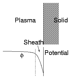
1.2.4 Plasma-Solid Boundaries (Elementary)
When a plasma is in contact with a solid, the solid acts as a
"sink" draining away the plasma. Recombination of electrons
and ions occur at surface. Then:
- Plasma is normally charged positively with respect to the
solid.
Figure 1.7: Plasma-Solid interface: Sheath
- There is a relatively thin region called the "sheath",
at the boundary of the plasma, where the main potential variation
occurs.
Reason for potential drop:
Different velocities of electrons and ions.
If there were no potential variation (E= 0) the electrons
and ions would hit the surface at the random rate
[This equation comes from elementary gas-kinetic theory. See problems
if not familiar.]
The mean speed ―v = √{ [8 T/(πm)]} ∼ √{ T/m}.
Because of mass difference electrons move ∼ √{ [(mi)/(me)]}
faster and hence would drain out of plasma faster. Hence, plasma
charges up enough that an electric field opposes electron escape
and reduces total electric current to zero.
Estimate of potential:
Ion escape flux 1/4 n′i―vi
Electron escape flux 1/4 n′e ―vi
Prime denotes values at solid surface.
Boltzmann factor applied to electrons:
|
n′e = n∞ exp[ e ϕs / Te ] |
| (1.26) |
where ϕs is solid potential relative to distant (∞)
plasma.
Since ions are being dragged out by potential assume n′i ∼ n∞ (Zi = 1).
[This is only approximately correct.]
Hence total current density out of plasma is
| |
|
|
qi |
1
4
|
n′i |
-
v
|
i
|
+ qe |
1
4
|
n′e |
-
v
|
e
|
|
| | (1.27) |
| |
|
|
e n∞
4
|
{ |
-
v
|
i
|
− exp | ⎡
⎣
|
e ϕs
Te
| ⎤
⎦
|
|
-
v
|
e
|
} |
| | (1.28) |
|
This must be zero so
| |
|
|
|
Te
e
|
ln| |
|
| = |
Te
e
|
|
1
2
|
ln | ⎛
⎝
|
Ti
Te
|
|
me
mi
| ⎞
⎠
|
|
| | (1.29) |
| |
|
|
Te
e
|
|
1
2
|
ln | ⎛
⎝
|
me
mi
| ⎞
⎠
|
[if Te = Ti.] |
| | (1.30) |
|
For hydrogen [( mi)/(me)] = 1800 so
1/2 ln[(me)/(mi)] = − 3.75.
The potential of the surface relative to plasma is approximately
−4 [(Te)/e].
[Note [(Te)/e] is just the electron temperature in electron-volts
expressed as a voltage.]
1.2.5 Thickness of the sheath
Crude estimates of sheath thickness can be obtained by assuming that
ion density is uniform. Then equation of potential is, as before,
|
|
d2 ϕ
d x2
|
= |
e n∞
ϵ0
|
| ⎡
⎣
|
exp | ⎛
⎝
|
eϕ
Te
| ⎞
⎠
|
− 1 | ⎤
⎦
|
|
| (1.31) |
We know the rough scale-length of solutions of this equation
is
|
λD = | ⎛
⎝
|
ϵ0Te
e2 n∞
| ⎞
⎠
|
1/2
|
the Debye Length. |
| (1.32) |
Actually our previous solution was valid only for |eϕ/Te| << 1 which is no longer valid.
When −eϕ/Te > 1 (as will be the case in the sheath). We can
practically ignore the electron density, in which case the solution
will continue only quadratically. One might expect, therefore, that
the sheath thickness is roughly given by an electric potential
gradient
extending sufficient distance to reach ϕS = − 4 [( Te)/e]
i.e.
distance x ∼ 4 λD
This is correct for the typical sheath thickness but not at all
rigorous.
1.3 The `Plasma Parameter'
Notice that in our development of Debye shielding we used nee as
the charge density and supposed that it could be taken as smooth and
continuous. However if the density were so low that there were less
than approximately one electron in the Debye shielding region this
approach would not be valid. Actually we have to address this problem
in 3-d by defining the `Plasma Parameter', ND, as
ND = Number of particles in the `Debye Sphere'.
|
= n . |
4
3
|
πλ3D | ⎛
⎝
|
∝ |
T3/2
n1/2
| ⎞
⎠
|
. |
| (1.34) |
If ND <~1 then the individual particles cannot be treated
as a smooth continuum. It will be seen later that this means that
collisions dominate the behaviour: i.e. short range correlation is
just
as important as the long range collective effects.
Often, therefore we add a further qualification of plasma:
|
ND >> 1 (Collective effects dominate over collisions) |
| (1.35) |
1.4 Summary
Plasma is an ionized gas in which collective effects dominate
over collisions.
|
[ λD << size , ND >> 1 .] |
| (1.36) |
1.5 Occurrence of Plasmas
Gas Discharges: Fluorescent Lights, Spark gaps, arcs, welding,
lighting
Controlled Fusion
Ionosphere: Ionized belt surrounding earth
Interplanetary Medium: Magnetospheres of planets and starts.
Solar Wind.
Stellar Astrophysics: Stars. Pulsars. Radiation-processes.
Ion Propulsion: Advanced space drives, etc.
& Space Technology Interaction of Spacecraft with environment
Gas Lasers: Plasma discharge pumped lasers:
CO2, He, Ne, HCN.
Materials Processing: Surface treatment for hardening. Crystal
Growing.
Semiconductor Processing: Ion beam doping, plasma etching &
sputtering.
Solid State Plasmas: Behavior of semiconductors.
For a figure locating different types of plasma in the plane of
density versus temperature see for example Goldston and Rutherford
Introduction to Plasma Physics IOP Publishing, 1995, figure 1.3
page 9. Another is at http://www.plasmas.org/basics.htm
1.6 Different Descriptions of Plasma
- Single Particle Approach. (Incomplete in itself). Eq. of Motion.
- Kinetic Theory. Boltzmann Equation.
|
| ⎡
⎣
|
∂
∂t
|
+ v. |
∂
∂x
|
+ a . |
∂
∂v
| ⎤
⎦
|
f = |
∂f
∂t
| ⎞
⎠
|
col.
|
|
| (1.37) |
- Fluid Description. Moments, Velocity, Pressure, Currents, etc.
Uses of these.
Single Particle Solutions → Orbits
→ Kinetic Theory Solutions →
Transport Coefs.
→ Fluid Theory → Macroscopic Description
All descriptions should be consistent. Sometimes they are different
ways of
looking at the same thing.
1.6.1 Equations of Plasma Physics
1.6.2 Self Consistency
In solving plasma problems one usually has a `circular' system:
The problem is solved only when we have a model in which all parts are
self consistent. We need a `bootstrap' procedure.
Generally we have to do it in stages:
- Calculate Plasma Response (to given E,B)
- Get currents & charge densities
- Calculate E & B for j, p.
Then put it all together. This will become clearer by example as we
develop the subject.