HEAD

Chapter 2
Motion of Charged Particles in Fields

Plasmas are complicated because motions of electrons and ions are determined by the electric and magnetic fields but also change the fields by the currents they carry.

For now we shall ignore the second part of the problem and assume that Fields are Prescribed.

Even so, calculating the motion of a charged particle can be quite hard.

Equation of motion:

Rate of change of momentum

q
charge

(

E
E-field

v
velocity

B
B-field

)

Lorentz Force

(2.1)

Have to solve this differential equation, to get position r and velocity (v= · r) given E(r,t), B(r,t).

Approach: Start simple, gradually generalize.

2.1 Uniform B field, E = 0.

= q vÙB

(2.2)

2.1.1 Qualitatively

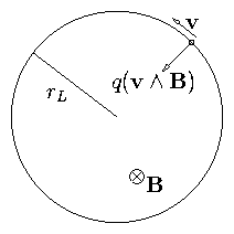
in the plane perpendicular to B:

Figure 2.1: Circular orbit in uniform magnetic field.

Accel. is perp to v so particle moves in a circle whose radius r_L is such as to satisfy

m r_L W² = m

v_^²

r_L

= |q |v_^ B

(2.3)

W is the angular (velocity) frequency

1st equality shows W² = v_^² /r_L² (r_L = v_^ / W)

Hence second gives m [(v_^)/(W)] W² = |q |v_^ B

i.e. W =

|q |B

(2.4)

Particle moves in a circular orbit with

angular velocity W =

|q |B

the "Cyclotron Frequency"

(2.5)

and radius r_l =

v_^

the "Larmor Radius.

(2.6)

2.1.2 By Vector Algebra

Particle Energy is constant. proof: take v. Eq. of motion then

m v.
×

v

= d
dt
æ
è 1
2
m v² ö
ø = q v. (vÙB) = 0 .
(2.7)
Parallel and Perpendicular motions separate. v_|| = constant because accel ( µ vÙB) is perpendicular to B.

Perpendicular Dynamics:

Take B in Ùz direction and write components

= q v_y B , m

= - q v_x B

(2.8)

Hence

××

= -

æ
è

ö
ø

v_x = - W² v_x

(2.9)

Solution: v_x = v_^ cosWt (choose zero of time)

Substitute back:

v_y =

= -

|q |

v_^ sinWt

(2.10)

Integrate:

x = x₀ +

v_^

sinWt , y = y₀ +

|q |

v_^

cosWt

(2.11)

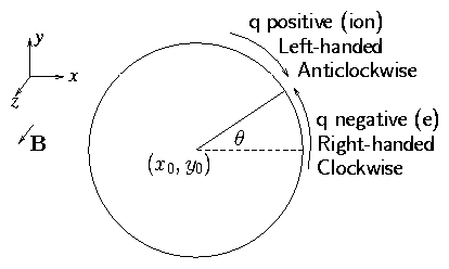
Figure 2.2: Gyro center (x₀,y₀) and orbit

This is the equation of a circle with center r₀ = (x₀, y₀) and radius r_L = v_^/ W: Gyro Radius. [Angle is q = Wt]

Direction of rotation is as indicated opposite for opposite sign of charge:

Ions rotate anticlockwise. Electrons clockwise about the magnetic field.

The current carried by the plasma always is in such a direction as to reduce the magnetic field.

This is the property of a magnetic material which is "Diagmagnetic".

When v_|| is non-zero the total motion is along a helix.

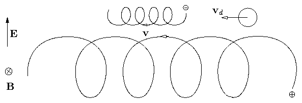
2.2 Uniform B and non-zero E

= q (E+ vÙB)

(2.12)

Parallel motion: Before, when E = 0 this was v_|| = const. Now it is clearly

q E_||

(2.13)

Constant acceleration along the field.

Perpendicular Motion

Qualitatively:

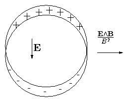
Figure 2.3: EÙB drift orbit

Speed of positive particle is greater at top than bottom so radius of curvature is greater. Result is that guiding center moves perpendicular to both E and B. It `drifts' across the field.

Algebraically: It is clear that if we can find a constant velocity v_d that satisfies

E+ v_d ÙB= 0

(2.14)

then the sum of this drift velocity plus the velocity

v_L =

[r_L e^iW(t-t₀)]

(2.15)

which we calculated for the E = 0 gyration will satisfy the equation of motion.

Take ÙB the above equation:

0 = EÙB+ (v_d ÙB) ÙB=EÙB+ (v_d . B) B- B² v_d

(2.16)

so that

v_d =

EÙB

B²

(2.17)

does satisfy it.

Hence the full solution is

v_||
parallel

v_d
cross-field drift

v_L
Gyration

(2.18)

where

q E_||

(2.19)

and

v_d (eq 2.17) is the "E × B drift" of the gyrocenter.

Comments on E × B drift:

It is independent of the properties of the drifting particle (q, m, v, whatever).
Hence it is in the same direction for electrons and ions.
Underlying physics for this is that in the frame moving at the E × B drift E = 0. We have `transformed away' the electric field.
Formula given above is exact except for the fact that relativistic effects have been ignored. They would be important if v_d ~ c.

2.2.1 Drift due to Gravity or other Forces

Suppose particle is subject to some other force, such as gravity. Write it F so that

= F + q vÙB = q (

F+ vÙB)

(2.20)

This is just like the Electric field case except with F/q replacing E.

The drift is therefore

v_d =

F ÙB

B²

(2.21)

In this case, if force on electrons and ions is same, they drift in opposite directions.

This general formula can be used to get the drift velocity in some other cases of interest (see later).

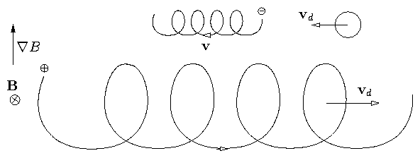
2.3 Non-Uniform B Field

If B-lines are straight but the magnitude of B varies in space we get orbits that look qualitatively similar to the E ^ B case:

Figure 2.4: ÑB drift orbit

Curvature of orbit is greater where B is greater causing loop to be small on that side. Result is a drift perpendicular to both B and ÑB. Notice, though, that electrons and ions go in opposite directions (unlike EÙB).

Algebra

We try to find a decomposition of the velocity as before into v = v_d + v_L where v_d is constant.

We shall find that this can be done only approximately. Also we must have a simple expression for B. This we get by assuming that the Larmor radius is much smaller than the scale length of B variation i.e.,

r_L << B/ |Ñ B |

(2.22)

in which case we can express the field approximately as the first two terms in a Taylor expression:

B @ B₀ + (r. Ñ ) B

(2.23)

Then substituting the decomposed velocity we get:

= q (vÙB) = q [ v_L ÙB₀ + v_d ÙB₀ + (v_L + v_d) Ù(r. Ñ) B]

(2.24)

or 0

v_d ÙB₀ + v_L Ù(r. Ñ ) B+ v_d Ù(r. Ñ) B

(2.25)

Now we shall find that v_d/v_L is also small, like r| ÑB | /B. Therefore the last term here is second order but the first two are first order. So we drop the last term.

Now the awkward part is that v_L and r_L are periodic. Substitute for r = r₀ + r_L so

0 = v_d ÙB₀ + v_L Ù(r_L . Ñ ) B+ v_L Ù( r₀ . Ñ ) B

(2.26)

We now average over a cyclotron period. The last term is µ e^-iWt so it averages to zero:

0 = v_d ÙB+ áv_L Ù(r_L . Ñ ) Bñ .

(2.27)

To perform the average use

r_L = ( x_L , y_L)

v_^

æ
è

sinWt ,

|q |

cosWt

ö
ø

(2.28)

v_L = (

)

v_^

æ
è

cosWt ,

-q

|q |

sinWt

ö
ø

(2.29)

So [ v_L Ù(r. Ñ ) B]_x

v_y y

(2.30)

[ v_L Ù( r. Ñ ) B]_y

-v_x y

(2.31)

(Taking ÑB to be in the y-direction).

Then

áv_y y ñ

- ácosWt sinWt ñ

v_^²

= 0

(2.32)

áv_x y ñ

|q |

ácosWt cosWt ñ

v_^²

|q |

(2.33)

áv_L Ù(r. Ñ ) Bñ = -

|q |

v_^²

Ñ B

(2.34)

Substitute in:

0 = v_d ÙB-

|q |

v_^²

Ñ B

(2.35)

and solve as before to get

v_d =

æ
è

-1

|q |

v_^²

2 W

Ñ B

ö
ø

ÙB

B²

|q |

v_^²

2 W

BÙÑ B

B²

(2.36)

or equivalently

v_d =

mv_^²

2 B

BÙÑ B

B²

(2.37)

This is called the `Grad B drift'.

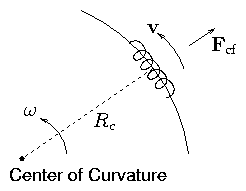
2.4 Curvature Drift

When the B-field lines are curved and the particle has a velocity v_|| along the field, another drift occurs.

Figure 2.5: Curvature and Centrifugal Force

Take |B| constant; radius of curvature R_e.

To 1st order the particle just spirals along the field.

In the frame of the guiding center a force appears because the plasma is rotating about the center of curvature.

This centrifugal force is F_cf

F_cf = m

v_||²

R_c

pointing outward

(2.38)

as a vector

F_cf = m v_||²

R_c

R_c²

(2.39)

[There is also a coriolis force 2m(w Ùv) but this averages to zero over a gyroperiod.]

Use the previous formula for a force

v_d =

F_cf ÙB

B²

m v_||²

q B²

R_c ÙB

R_c²

(2.40)

This is the "Curvature Drift".

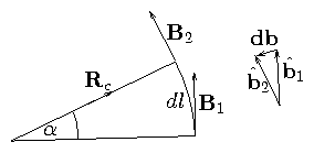
It is often convenient to have this expressed in terms of the field gradients. So we relate R_c to ÑB etc. as follows:

Figure 2.6: Differential expression of curvature

(Carets denote unit vectors)

From the diagram

db =

= -

(2.41)

and

d l = µ R_c

(2.42)

d b

d l

= -

R_c

= -

R_c

R_c²

(2.43)

But (by definition)

d b

d l

= (

. Ñ )

(2.44)

So the curvature drift can be written

v_d =

m v_||²

R_c

R_c²

B²

mv_||²

BÙ(

. Ñ )

B²

(2.45)

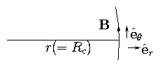
2.4.1 Vacuum Fields

Relation between Ñ B & R_c drifts

The curvature and ÑB are related because of Maxwell's equations, their relation depends on the current density j. A particular case of interest is j=0: vacuum fields.

Figure 2.7: Local polar coordinates in a vacuum field

Ñ ÙB= 0 (static case)

(2.46)

Consider the z-component

0 = ( Ñ ÙB)_z

¶r

(r B_q ) (B_r = 0 by choice).

(2.47)

¶B_q

¶r

B_q

(2.48)

or, in other words,

( Ñ B )_r = -

R_c

(2.49)

[Note also 0 = (Ñ ÙB)_q = ¶B_q/¶z : (Ñ B )_z = 0]

and hence (Ñ B)_perp = - B R_c/R_c².

Thus the grad B drift can be written:

v_ÑB =

mv_^²

2 q

BÙÑ B

B³

mV_^²

2 q

R_c ÙB

R_c² B²

(2.50)

and the total drift across a vacuum field becomes

v_R + v_ÑB =

æ
è

mv_||² +

mv_^²

ö
ø

R_c ÙB

R_c² B²

(2.51)

Notice the following:

R_c & ÑB drifts are in the same direction.
They are in opposite directions for opposite charges.
They are proportional to particle energies
Curvature « Parallel Energy (× 2)
ÑB « Perpendicular Energy
As a result one can very quickly calculate the average drift over a thermal distribution of particles because

á 1
2
m v_||² ñ

=

T
2

(2.52)

á 1
2
m v_^² ñ

=

T 2 degrees of freedom
(2.53)

Therefore

áv_R + v_ÑB ñ = 2T
q
R_c ÙB
R_c² B²
æ
ç
è = 2T
q

BÙ æ
è
^

b

. Ñ ö
ø
^

b

B²
ö
÷
ø
(2.54)

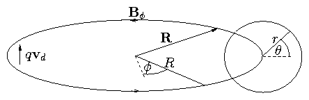
2.5 Interlude: Toroidal Confinement of Single Particles

Since particles can move freely along a magnetic field even if not across it, we cannot obviously confine the particles in a straight magnetic field. Obvious idea: bend the field lines into circles so that they have no ends.

Figure 2.8: Toroidal field geometry

Problem

Curvature & ÑB drifts

v_d

æ
è

mv_||² +

mv_^²

ö
ø

R ÙB

R² B²

(2.55)

|v_d |

æ
è

mv_||² +

mv_^²

ö
ø

(2.56)

Figure 2.9: Charge separation due to vertical drift

Ions drift up. Electrons down. There is no confinement. When there is finite density things are even worse because charge separation occurs ® E ® E ÙB ® Outward Motion.

2.5.1 How to solve this problem?

Consider a beam of electrons v_|| ¹ 0 v_^ = 0. Drift is

v_d =

mv_||²

B_TR

(2.57)

What B_z is required to cancel this?

Adding B_z gives a compensating vertical velocity

v = v_||

B_z

B_T

for B_z << B_T

(2.58)

We want total

v_z = 0 = v_||

B_z

B_T

mv_||²

B_TR

(2.59)

So B_z = - mv_||/ Rq is the right amount of field.

Note that this is such as to make

r_L (B_z) =

|mv_|| |

|q B_z |

= R .

(2.60)

But B_z required depends on v_|| and q so we can't compensate for all particles simultaneously.

Vertical field along cannot do it.

2.5.2 The Solution: Rotational Transform

Figure 2.10: Tokamak field lines with rotational transform

Toroidal Coordinate system (r, q, f) (minor radius, poloidal angle, toroidal angle), see figure 2.8.

Suppose we have a poloidal field B_q

Field Lines become helical and wind around the torus: figure 2.10.

In the poloidal cross-section the field describes a circle as it goes round in f.

Equation of motion of a particle exactly following the field is:

d q

B_q

B_f

v_f =

B_q

B_f

v_|| =

B_q

v_||

(2.61)

and

r = constant.

(2.62)

Now add on to this motion the cross field drift in the Ùz direction.

Figure 2.11: Components of velocity

d q

B_q

v_|| + v_d cosq

(2.63)

v_d sinq

(2.64)

Take ratio, to eliminate time:

u_d sinq

B_q

v_|| +v_d cosq

(2.65)

Take B_q, B, v_||, v_d to be constants, then we can integrate this orbit equation:

[ lnr ] = [ - ln|

B_q v_||

+ v_d cosq|] .

(2.66)

Take r = r₀ when cosq = 0 (q = [( p)/2]) then

r = r₀ /

é
ë

1 +

Bv_d

b_q v_||

cosq

ù
û

(2.67)

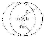
If [( Bv_d)/(B_q v_|| )] << 1 this is approximately

r = r₀ - Dcosq

(2.68)

where D = [(Bv_d)/(B_q v_|| )] r₀

This is approximately a circular orbit shifted by a distance D:

Figure 2.12: Shifted, approximately circular orbit

Substitute for v_d

r₀

B_q

(mv_||² +

mv_^²)

v_||

B_f R

(2.69)

q B_q

mv_||² +

mv_^²

v_||

r_p

(2.70)

If v_^ = 0

D =

mv_||

q B_q

r₀

= r_Lq

r₀

(2.71)

where r_Lq is the Larmor Radius in a field B_q ×r / R.

Provided D is small, particles will be confined. Obviously the important thing is the poloidal rotation of the field lines: Rotational Transform.

Rotational Transform

rotational transform

poloidal angle

1 toroidal rotation

(2.72)

( transform / 2p = )

i º

poloidal angle

toroidal angle

(2.73)

(Originally, i was used to denote the transform. Since about 1990 it has been used to denote the transform divided by 2p which is the inverse of the safety factor.)

`Safety Factor'

`q_s¢ =

toroidal angle

poloidal angle

(2.74)

Actually the value of these ratios may vary as one moves around the magnetic field. Definition strictly requires one should take the limit of a large no. of rotations.

q_s is a topological number: number of rotations the long way per rotation the short way.

Cylindrical approx.:

q_s =

r B_f

R B_q

(2.75)

In terms of safety factor the orbit shift can be written

|D| = r_{L q}

= r_{L f}

B_f r

B_q R

= r_L q_s

(2.76)

(assuming B_f >> B_q).

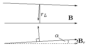
2.6 The Mirror Effect of Parallel Field Gradients: E = 0, ÑB ||B

Figure 2.13: Basis of parallel mirror force

In the above situation there is a net force along B.

Force is

< F_|| >

- |q vÙB| sina = - |q |v_^ B sina

(2.77)

sina

- B_r

(2.78)

Calculate B_r as function of B_z from Ñ . B = 0.

Ñ . B=

¶r

(rB_r) +

¶z

B_z = 0 .

(2.79)

Hence

rB_r = -

ó
õ

¶B_z

¶z

(2.80)

Suppose r_L is small enough that [(¶B_z)/(¶z)] @ const.

[ r B_r]₀^r_L @

ó
õ

r_L

0

r dr

¶B_z

¶z

= -

r_L²

¶B_z

¶z

(2.81)

B_r(r_L) = -

r_L

¶B_z

¶z

(2.82)

sina = -

B_r

= +

r_L

¶B_z

¶z

(2.83)

Hence

< F_|| > = - |q |

v_^ r_L

¶B_z

¶z

= -

mv_^²

¶B_z

¶z

(2.84)

As particle enters increasing field region it experiences a net parallel retarding force.

Define Magnetic Moment

m º

m v_^² / B .

(2.85)

Note this is consistent with loop current definition

m = A I = pr_L² .

|q |v_^

2 pr_L

|q |r_L v_^

(2.86)

Force is F_|| = m . Ñ_|| B

This is force on a `magnetic dipole' of moment m.

F_|| = m . Ñ_|| B

(2.87)

Our m always points along B but in opposite direction.

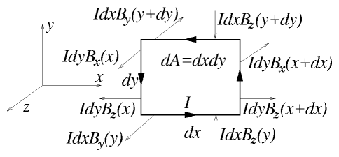
2.6.1 Force on an Elementary Magnetic Moment Circuit

Consider a plane rectangular circuit carrying current I having elementary area dxdy = dA. Regard this as a vector pointing in the z direction dA. The force on this circuit in a field B(r) is F such that

F_x

Idy [B_z (x+dx) - B_z(x)] = I dydx

¶B_z

¶x

(2.88)

F_y

-I dx [B_z (y+dy) - B_z(y)] = I dydx

¶B_z

¶y

(2.89)

F_z

- I dx [B_y (y+dy) - B_y(y)] - I dy[B_x(x+dx) - B_x(x)]

(2.90)

- I dxdy

é
ë

¶B_x

¶x

¶B_y

¶y

ù
û

= I dydx

¶B_z

¶z

(2.91)

(Using Ñ . B = 0).

Hence, summarizing: F = I dydx Ñ B_z. Now define m = I dA = I dydx Ùz and take it constant. Then clearly the force can be written

F = Ñ (B. m ) [ Strictly = (Ñ B) . m]

(2.92)

m is the (vector) magnetic moment of the circuit.

The shape of the circuit does not matter since any circuit can be considered to be composed of the sum of many rectangular circuits. So in general

m = I dA

(2.93)

and force is

F = Ñ (B. m) (m constant),

(2.94)

We shall show in a moment that |m | is constant for a circulating particle, regard as an elementary circuit. Also, m for a particle always points in the -B direction. [Note that this means that the effect of particles on the field is to decrease it.] Hence the force may be written

F = - mÑ B

(2.95)

This gives us both:

Magnetic Mirror Force:

F_|| = -mÑ_||B
(2.96)
and
Grad B Drift:

v_ÑB = 1
q
F ÙB
B²
= m
q
BÙÑ B
B²
.
(2.97)

2.6.2 m is a constant of the motion

`Adiabatic Invariant'

Proof from F_||

Parallel equation of motion

dv_||

= F_|| = - m

(2.98)

m v_||

dv_||

(

m v_||² ) = - mv_z

= - m

(2.99)

(

m v_||²) + m

= 0 .

(2.100)

Conservation of Total KE

(

mv_||² +

mv_^² ) = 0

(2.101)

(

mv_||² + mB) = 0

(2.102)

Combine

(mB) - m

= 0

(2.103)

d m

= 0 As required

(2.104)

Angular Momentum

of particle about the guiding center is

r_L mv_^

mv_^

|q |B

m v_^ =

|q |

mv_^²

(2.105)

|q |

m .

(2.106)

Conservation of magnetic moment is basically conservation of angular momentum about the guiding center.

Proof direct from Angular Momentum

Consider angular momentum about G.C. Because q is ignorable (locally) Canonical angular momentum is conserved.

p = [ r Ù( m v+ q A) ]_z conserved.

(2.107)

Here A is the vector potential such that B = Ñ ÙA

the definition of the vector potential means that

B_z

¶(rA_q))

¶r

(2.108)

Þ r_L A_q (r_L)

ó
õ

r_L

0

r . B_z dr =

r_L²

B_z =

|q |

(2.109)

Hence

- q

|q |

r_L v_^ m + q

|q|

(2.110)

|q |

m m.

(2.111)

So p = const « m = constant.

Conservation of m is basically conservation of angular momentum of particle about G.C.

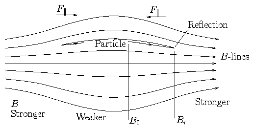
2.6.3 Mirror Trapping

Figure 2.14: Magnetic Mirror

F_|| may be enough to reflect particles back. But may not!

Let's calculate whether it will:

Suppose reflection occurs.

At reflection point v_||r = 0.

Energy conservation

m (v_^0² + v_||0²) =

m v_^r²

(2.112)

m conservation

m v_^0²

B₀

m v_^r²

B_r

(2.113)

Hence

v_^0² + v_||0²

B_r

B₀

v_^0²

(2.114)

B₀

B_r

v_^0²

v_^0² + v_||o²

(2.115)

2.6.4 Pitch Angle q

tanq

v_^

v_||

(2.116)

B₀

B_r

v_^0²

v_^0² +v_||0²

= sin² q₀

(2.117)

So, given a pitch angle q₀, reflection takes place where B₀/B_r = sin²q₀.

If q₀ is too small no reflection can occur.

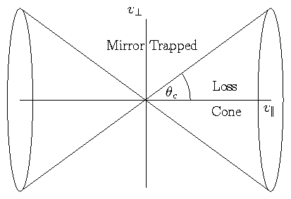
Critical angle q_c is obviously

q_c = sin^-1 (B₀ / B₁)^¹/₂

(2.118)

Loss Cone is all q < q_c.

Figure 2.15: Critical angle q_c divides velocity space into a loss-cone and a region of mirror-trapping

Importance of Mirror Ratio: R_m = B₁ / B₀.

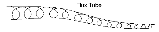
2.6.5 Other Features of Mirror Motions

Flux enclosed by gyro orbit is constant.

pr_L² B =

pm² v_^²

q² B²

(2.119)

2 pm

q²

mv_^²

(2.120)

2 pm

q²

m = constant.

(2.121)

Figure 2.16: Flux tube described by orbit

Note that if B changes `suddenly' m might not be conserved.

Basic requirement

r_L << B / |ÑB |

(2.122)

Slow variation of B (relative to r_L).

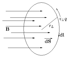
2.7 Time Varying B Field (E inductive)

Figure 2.17: Particle orbits round B so as to perform a line integral of the Electric field

Particle can gain energy from the inductive E field

ÑÙE

¶B

¶t

(2.123)

ó
(ç)
õ

E.dl

ó
õ

. ds = -

d F

d t

(2.124)

Hence work done on particle in 1 revolution is

dw = -

ó
(ç)
õ

|q|E. dl = + |q |

ó
õ

. ds = + |q |

d F

= |q |

pr_L²

(2.125)

(dl and v_^ q are in opposition directions).

æ
è

m v_^²

ö
ø

|q |

pr _L² =

2 p

|q |B

m v_^²

(2.126)

2 p

|W|

(2.127)

Hence

æ
è

m v_^²

ö
ø

|W|

2 p

æ
è

mv_^²

ö
ø

= m

(2.128)

but also

æ
è

mv_^²

ö
ø

( mB ) .

(2.129)

Hence

= 0 .

(2.130)

Notice that since F = [(2 pm)/(q² )] m, this is just another way of saying that the flux through the gyro orbit is conserved.

Notice also energy increase. Method of `heating'. Adiabatic Compression.

2.8 Time Varying E-field (E, B uniform)

Recall the EÙB drift:

v_{E ÙB} =

EÙB

B²

(2.131)

when E varies so does v_{E ÙB}. Thus the guiding centre experiences an acceleration

E ÙB

æ
è

EÙB

B²

ö
ø

(2.132)

In the frame of the guiding centre which is accelerating, a force is felt.

F_a = - m

æ
è

EÙB

B²

ö
ø

(Pushed back into seat! -ve.)

(2.133)

This force produces another drift

v_D

F_a ÙB

B²

qB²

æ
è

EÙB

B²

ö
ø

ÙB

(2.134)

( ( E. B) B- B²E)

(2.135)

q B²

(2.136)

This is called the `polarization drift'.

v_D = v_{E ÙB}

v_p =

EÙB

B²

q B²

(2.137)

E ÙB

B²

(2.138)

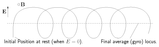
Figure 2.18: Suddenly turning on an electric field causes a shift of the gyrocenter in the direction of force. This is the polarization drift.

Start-up effect: When we `switch on' an electric field the average position (gyro center) of an initially stationary particle shifts over by ~ ¹/₂ the orbit size. The polarization drift is this polarization effect on the medium.

Total shift due to v_p is

ó
õ

v_p dt =

q B²

ó
õ

dt =

q B²

[ DE_^ ] .

(2.139)

2.8.1 Direct Derivation of [(dE)/dt] effect: `Polarization Drift'

Consider an oscillatory field E = Ee^-iwt (^r₀B)

q ( E+ vÙB)

(2.140)

q ( Ee^-iwt + vÙB)

(2.141)

Try for a solution in the form

v= v_D e^-iwt + v_L

(2.142)

where, as usual, v_L satisfies m · v_L = q v_L ÙB

Then

(1) m(-i wv_D = q ( E+ v_D ÙB) xl^{-i wt}

(2.143)

Solve for v_D: Take ÙB this equation:

(2) - m i w( v_D ÙB) = q ( EÙB+ ( B² . v|D ) B-B² v_D )

(2.144)

add m i w×(1) to q ×(2) to eliminate v_D ÙB.

m² w² v_D + q² ( EÙB- B² v_D ) = mi wq E

(2.145)

or: v_D

é
ë

1 -

m² w²

q² B²

ù
û

= -

miw

qB²

E+

EÙB

B²

(2.146)

i.e. v_D

é
ë

1 -

w²

W²

ù
û

= -

iwq

WB |q |

E+

EÙ B

B²

(2.147)

Since -iw« [(¶)/(¶t)] this is the same formula as we had before: the sum of polarization and EÙB drifts except for the [1 - w²W²] term.

This term comes from the change in v_D with time (accel).

Thus our earlier expression was only approximate. A good approx if w << W.

2.9 Non Uniform E (Finite Larmor Radius)

= q ( E(r) + vÙB)

(2.148)

Seek the usual soltuion v = v_D + v_g.

Then average out over a gyro orbit

ám

dv_D

0 = áq ( E(r) + vÙB) ñ

(2.149)

q [ áE(r) ñ+ v_D ÙB]

(2.150)

Hence drift is obviously

v_D =

áE(r) ñÙB

B²

(2.151)

So we just need to find the average E field experienced.

Expand E as a Taylor series about the G.C.

E(r) = E₀ +( r. Ñ) E+

æ
è

x²¶²

2!¶x²

y²

¶²

¶y²

ö
ø

E+ cross terms + .

(2.152)

(E.g. cross terms are x y [(¶²)/(¶x ¶y)]E).

Average over a gyro orbit: r = r_L (cosq, sinq,0).

Average of cross terms = 0.

Then

áE(r) ñ = E+ ( ár_L ñ. Ñ) E+

ár_L²ñ

Ñ² E.

(2.153)

linear term ár_Lñ = 0. So

áE(r)ñ @ E+

r_L²

Ñ² E

(2.154)

Hence EÙB with 1st finite-Larmor-radius correction is

v_{E ÙB} =

æ
è

1 +

r_L²

Ñ²

ö
ø

EÙB

B²

(2.155)

[Note: Grad B drift is a finite Larmor effect already.]

Second and Third Adiabatic Invariants

There are additional approximately conserved quantities like m in some geometries.

2.10 Summary of Drifts

v_E

EÙB

B²

Electric Field

(2.156)

v_F

F ÙB

B²

General Force

(2.157)

v_E

æ
è

1 +

r_L²

Ñ²

ö
ø

EÙB

B²

Nonuniform E

(2.158)

v_ÑB

mv_^²

BÙÑ B

B³

Grad B

(2.159)

v_R

mv_||²

R_c ÙB

R_c² B²

Curvature

(2.160)

v_R + v_ÑB

æ
è

mv_||² +

m v_^²

ö
ø

R_c ÙB

R_c² B²

Vacuum Fields.

(2.161)

v_p

|q |

|W|B

Polarization

(2.162)

Mirror Motion

m º

mv_^²

is constant

(2.163)

Force is F = - mÑB.

HEAD

Chapter 2 Motion of Charged Particles in Fields

2.1 Uniform B field, E = 0.

2.1.1 Qualitatively

2.1.2 By Vector Algebra

2.2 Uniform B and non-zero E

2.2.1 Drift due to Gravity or other Forces

2.3 Non-Uniform B Field

Algebra

2.4 Curvature Drift

2.4.1 Vacuum Fields

2.5 Interlude: Toroidal Confinement of Single Particles

2.5.1 How to solve this problem?

2.5.2 The Solution: Rotational Transform

Rotational Transform

`Safety Factor'

2.6 The Mirror Effect of Parallel Field Gradients: E = 0, ÑB ||B

2.6.1 Force on an Elementary Magnetic Moment Circuit

2.6.2 m is a constant of the motion

Proof from F||

Angular Momentum

Proof direct from Angular Momentum

2.6.3 Mirror Trapping

2.6.4 Pitch Angle q

2.6.5 Other Features of Mirror Motions

2.7 Time Varying B Field (E inductive)

2.8 Time Varying E-field (E, B uniform)

2.8.1 Direct Derivation of [(dE)/dt] effect: `Polarization Drift'

2.9 Non Uniform E (Finite Larmor Radius)

2.10 Summary of Drifts

Chapter 2
Motion of Charged Particles in Fields

Proof from F_||