Chapter 5
Electromagnetic Waves in Plasmas
5.1 General Treatment of Linear Waves in Anisotropic Medium
Start with general approach to waves in a linear Medium: Maxwell:
|
∇ ∧B= μo j + |
1
c2
|
|
∂E
∂t
|
; ∇ ∧E
= − |
∂B
∂t
|
|
| (5.1) |
we keep all the medium's response explicit in j. Plasma
is (infinite and) uniform so we Fourier analyze in space and
time. That is we seek a solution in which all variables go like
|
expi ( k . x − ωt ) [real part of] |
| (5.2) |
It is really the linearised equations which we treat this way;
if there is some equilibrium field OK but the equations above mean
implicitly the perturbations B, E, j, etc.
Fourier analyzed:
|
i k ∧B= μo j+ |
−iω
c2
|
E ; i k ∧E
= i ωB
|
| (5.3) |
Eliminate B by taking k∧ second eq. and
ω× 1st
|
i k ∧(k ∧E) = ωμo j− |
i ω2
c2
|
E |
| (5.4) |
So
|
k ∧(k ∧E) + |
ω2
c2
|
E+ i ωμo j= 0 |
| (5.5) |
Now, in order to get further we must have some relationship
between j and E(k,ω). This will have to
come from solving the plasma equations but for now we can
just write the most general linear relationship
j and E as
σ is the `conductivity tensor'. Think of this
equation as a matrix e.g.:
|
| ⎛
⎜
⎜
⎜
⎝
|
|
| ⎞
⎟
⎟
⎟
⎠
|
= | ⎛
⎜
⎜
⎜
⎝
|
|
| ⎞
⎟
⎟
⎟
⎠
|
| ⎛
⎜
⎜
⎜
⎝
|
|
| ⎞
⎟
⎟
⎟
⎠
|
|
| (5.7) |
This is a general form of Ohm's Law. Of course if the
plasma (medium) is isotropic (same in all directions)
all off-diagonal σ′s are zero and one gets
j
= σE.
Thus
|
k (k . E) − k2 E+ |
ω2
c2
|
E+ i ωμoσ . E= 0 |
| (5.8) |
Recall that in elementary E&M, dielectric media are discussed
in terms of a dielectric constant ϵ and a "polarization"
of the medium, P, caused by modification of atoms.
Then
|
ϵ0 E= |
D
Displacement
|
− |
P
Polarization
|
and ∇ . D = |
ρext
external charge
|
|
| (5.9) |
and one writes
Our case is completely analogous, except we have chosen to
express the response of the medium in terms of current density,
j, rather than "polarization" P
For such a dielectric medium, Ampere's law would be written:
|
|
1
μo
|
∇ ∧B= jext + |
∂D
∂t
|
= |
∂
∂t
|
ϵϵ0 E, if jext = 0 , |
| (5.11) |
where the dielectric constant would be ϵ = 1 + χ.
Thus, the explicit polarization current can be expressed in the
form of an equivalent dielectric expression if
|
j+ ϵ0 |
∂E
∂t
|
= σ . E+ ϵ0 |
∂E
∂t
|
= |
∂
∂t
|
ϵ0 ϵ . E |
| (5.12) |
or
Notice the dielectric constant is a tensor because of
anisotropy.
The last two terms come from the RHS of Ampere's law:
If we were thinking in terms of a dielectric medium with
no explicit currents, only implicit (in ϵ) we would
write this [(∂)/(∂t)] (ϵϵ0 E);
ϵ the dielectric constant. Our medium is possibly
anisotropic so we need [(∂)/(∂t)] (ϵ0ϵ . E) dielectric tensor. The
obvious thing is therefore to define
|
ϵ = 1 + |
1
−iωϵ0
|
σ = 1 + |
i μo c2
ω
|
σ |
| (5.15) |
Then
|
k ( k . E) − k2 E+ |
ω2
c2
|
ϵ . E= 0 |
| (5.16) |
and we may regard ϵ (k, ω) as
the dielectric tensor.
Write the equation as a tensor multiplying E:
with
|
K= { k k − k2 1 + |
ω2
c2
|
ϵ } |
| (5.18) |
Again this is a matrix equation i.e.
3 simultaneous homogeneous eqs. for E.
|
| ⎛
⎜
⎜
⎜
⎝
|
|
| ⎞
⎟
⎟
⎟
⎠
|
| ⎛
⎜
⎜
⎜
⎝
|
|
| ⎞
⎟
⎟
⎟
⎠
|
= 0 |
| (5.19) |
In order to have a non-zero E solution we must have
This will give us an equation relating k and
ω, which tells us about the possible wavelengths
and frequencies of waves in our plasma.
5.1.1 Simple Case. Isotropic Medium
Take k in z direction
then write out the Dispersion tensor K.
|
K= |
k k
|
− |
k21
|
+ |
[(ω2)/(c2)]ϵ
|
|
|
Take determinant:
|
det | K | = | ⎛
⎝
|
− k2 + |
ω2
c2
|
ϵ | ⎞
⎠
|
2
|
|
ω2
c2
|
ϵ = 0 . |
| (5.24) |
Two possible types of solution to this dispersion relation:
(A)
|
⇒ | ⎛
⎜
⎜
⎜
⎜
⎜
⎝
|
|
| ⎞
⎟
⎟
⎟
⎟
⎟
⎠
|
| ⎛
⎜
⎜
⎜
⎝
|
|
| ⎞
⎟
⎟
⎟
⎠
|
= 0 ⇒ Ez = 0 . |
| (5.26) |
Electric field is transverse (E. k = 0)
Phase velocity of the wave is
This is just like a regular EM wave traveling in a medium
with refractive index
(B)
|
⇒ | ⎛
⎜
⎜
⎜
⎝
|
|
| ⎞
⎟
⎟
⎟
⎠
|
| ⎛
⎜
⎜
⎜
⎝
|
|
| ⎞
⎟
⎟
⎟
⎠
|
= 0 ⇒ Ex = Ey = 0 . |
| (5.30) |
Electric Field is Longitudinal
(E∧k = 0 ) E||k.
This has no obvious counterpart in optics etc. because
ϵ is not usually zero. In plasmas ϵ = 0
is a relevant solution. Plasmas can support
longitudinal waves.
5.1.2 General Case (k in z-direction)
|
K= |
ω2
c2
|
| ⎡
⎢
⎢
⎢
⎣
|
|
| ⎤
⎥
⎥
⎥
⎦
|
, | ⎛
⎝
|
N2 = |
k2 c2
ω2
| ⎞
⎠
|
|
| (5.31) |
When we take determinant we shall get a quadratic in N2 (for given
ω) provided ϵ is not explicitly dependent on
k. So for any ω there are two values of N2.
Two `modes'. The polarization E of these modes will be in
general partly longitudinal and partly transverse.
The point: separation into distinct longitudinal and
transverse modes is not possible in anisotropic media (e.g.
plasma with Bo).
All we have said applies to general linear medium (crystal,
glass, dielectric, plasma). Now we have to get the correct
expression for σ and hence ϵ by
analysis of the plasma (fluid) equations.
5.2 High Frequency Plasma Conductivity
We want, now, to calculate the current for given (Fourier)
electric field E(k,ω), to get the conductivity,
σ. It won't be the same as the DC conductivity
which we calculated before (for collisions) because the
inertia of the species will be important. In fact,
provided
we can ignore collisions altogether. Do this for simplicity,
although this approach can be generalized.
Also, under many circumstances we can ignore the pressure
force −∇p. In general will be true if
[(ω)/k] >> vte,i
Remember that we are dealing with uniform steady equilibrium
(suffix 0), so the equilibrium has zero electric field
E0=−∇ϕ0=0, (and pressure gradient ∇p0=0,) so
there is zero equilibrium perpendicular velocity, and we also take
v||0=0. The equilibrium is at rest. Also the wave is a
small perturbation to this equilibrium, which formally we could denote
with suffix 1, and we keep only first order quantities in the wave
equations. This gives a manageable problem with wide applicability.
We usually drop the suffixes once we've formulated the problem,
recognizing that B and n usually mean the equilibrium quantities
and varying things are the wave quantities.
Approximations:
5.2.1 Zero B-field case
To start with take B0 = 0: Plasma isotropic
Momentum equation (for electrons first)
|
mn | ⎡
⎣
|
∂v
∂t
|
+ ( v. ∇ )v | ⎤
⎦
|
= n q E |
| (5.34) |
Notice the characteristic of the cold plasma approx. that we can
cancel n from this equation and on linearizing get essentially the
single particle equation.
The equation can be solved for given ω as
and the current (due to this species, electrons) is
So the conductivity is
and the dielectric constant is
|
ϵ = 1 + |
i
ωϵ0
|
σ = 1 − | ⎛
⎝
|
nq2
m ϵ0
| ⎞
⎠
|
|
1
ω2
|
= 1 + χ |
| (5.39) |
Longitudinal Waves (B0 = 0)
Dispersion relation we know is
|
ϵ = 0 = 1 − | ⎛
⎝
|
n q2
m ϵ0
| ⎞
⎠
|
|
1
ω2
|
|
| (5.40) |
[Strictly, the ϵ we want here is the total ϵ
including both electron and ion contributions to the
conductivity.
But
|
|
σe
σi
|
≅ |
mi
me
|
(for z = 1) |
| (5.41) |
so to a first approximation, ignore ion motions.]
Solution
|
ω2 = | ⎛
⎝
|
ne qe2
me ϵ0
| ⎞
⎠
|
. |
| (5.42) |
In this approximation longitudinal oscillations of the electron
fluid have a single unique frequency:
|
ωp = | ⎛
⎝
|
ne e2
me ϵ0
| ⎞
⎠
|
1/2
|
. |
| (5.43) |
This is called the `Plasma Frequency' (more properly
ωpe the `electron' plasma frequency).
If we allow for ion motions we get an ion
conductivity
and hence
| |
|
|
1 + |
i
ωϵ0
|
( σe + σi ) = 1 − | ⎛
⎝
|
ne qe2
ϵ0 me
|
+ |
ni qi2
ϵ0 mi
| ⎞
⎠
|
|
1
ω2
|
|
| | (5.45) |
| |
|
| |
|
where
|
ωpi ≡ | ⎛
⎝
|
ni qi2
ϵ0 mi
| ⎞
⎠
|
1/2
|
|
| (5.46) |
is the `Ion Plasma Frequency'.
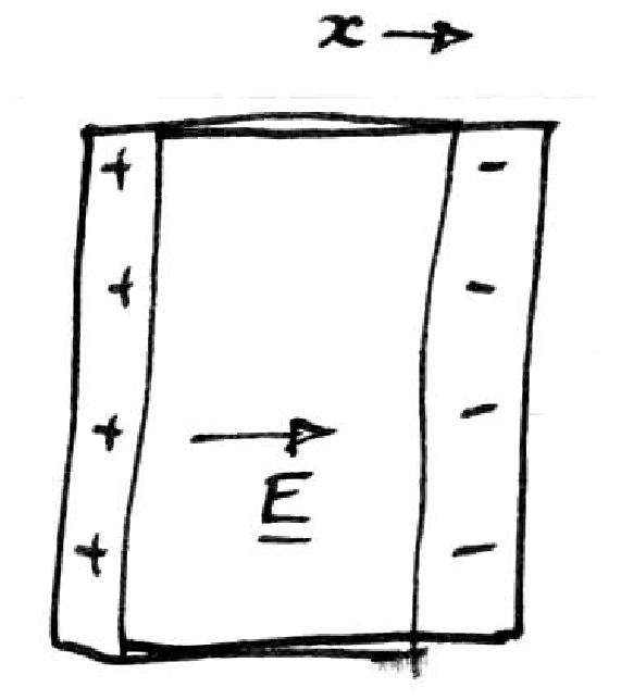
Simple Derivation of Plasma Oscillations
Figure 5.1: Slab derivation of plasma oscillations
Take ions stationary; perturb a slab of plasma by shifting
electrons a distance x.
Charge built up is neq x per unit area.
Hence electric field generated
Equation of motion of electrons
|
me |
dv
dt
|
= − |
ne qe2 x
ϵ0
|
; |
| (5.48) |
i.e.
|
|
d2x
dt2
|
+ | ⎛
⎝
|
ne qe2
ϵ0 me
| ⎞
⎠
|
x = 0 |
| (5.49) |
Simple harmonic oscillator with frequency
|
ωpe = | ⎛
⎝
|
ne qe2
ϵ0 me
| ⎞
⎠
|
1/2
|
Plasma Frequency. |
| (5.50) |
The Characteristic Frequency of Longitudinal Oscillations
in a plasma.
Notice
- ω = ωp for all k in this approx.
- Phase velocity [(ω)/k] can have any value.
- Group velocity of wave, which is the velocity at which
information/energy travel is
In a way, these oscillations can hardly be thought of as a
`proper' wave because they do not transport energy or information.
(In Cold Plasma Limit). [Nevertheless they do emerge from the
wave analysis and with less restrictive approximations do have finite
vg.]
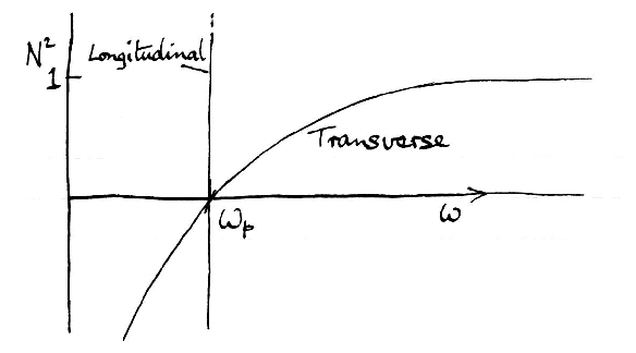
Transverse Waves (B0 = 0)
Dispersion relation:
or
| |
|
|
|
k2 c2
ω2
|
= ϵ = 1 −( ωpe2 + ωpi2 ) / ω2 |
| |
| |
|
| | (5.53) |
|
Figure 5.2: Unmagnetized plasma transverse wave.
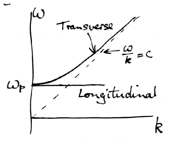
Figure 5.3: Alternative dispersion plot.
Alternative expression:
|
− k2 + |
ω2
c2
|
− |
ωp2
c2
|
= 0 |
| (5.54) |
which implies
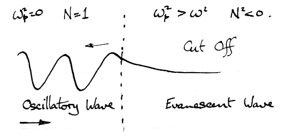
5.2.2 Meaning of Negative N2: Cut Off
When N2 < 0 (i.e. for ω < ωp), N is
pure imaginary and hence so is k for real ω.
Thus the wave we have found goes like
i.e. its space dependence is exponential not oscillatory.
Such a wave is said to be `Evanescent' or `Cut Off'.
It does not truly propagate through the medium but just damps
exponentially.
Example:
Figure 5.4: Wave behaviour at cut-off.
A wave incident on a plasma with ωp2 > ω2 is simply
reflected, no energy is transmitted through the plasma.
5.3 Cold Plasma Waves (Magnetized Plasma)
Objective: calculate ϵ, K,
k(ω), using known plasma equations.
Approximation: Ignore thermal motion of particles.
Applicability: Most situations where (1) plasma pressure and
(2) absorption are negligible. Generally requires wave
phase velocity >> vthermal.
5.3.1 Derivation of Dispersion Relation
Can "derive" the cold plasma approx from fluid plasma equations.
It is simpler just to say that all particles (of a specific species)
just move together obeying Newton's 2nd law:
Take the background plasma to have E0 = 0,
B
= B0 and zero velocity. Then all motion is due to the wave
and also the wave's magnetic field can be ignored provided the
particle speed stays small. (This is a linearization).
where v, E ∝ expi (k . x − ωt) are
wave quantities.
Substitute [(∂)/(∂t)] → − i ω
and write out equations.
Choose axes such that B0 = B0 (0,0,1).
Solve for v in terms of E.
| |
|
|
|
q
m
|
| ⎛
⎝
|
i ωEx − ΩEy
ω2 − Ω2
| ⎞
⎠
|
|
| |
| |
|
|
|
q
m
|
| ⎛
⎝
|
ΩEx + i ωEy
ω2 − Ω2
| ⎞
⎠
|
|
| | (5.61) |
| |
|
| |
|
where Ω = [(q B0)/m] is the gyrofrequency but
its sign is that of the charge on the particle species
under consideration.
Since the current is j
= q vn = σ . E
we can identify the conductivity tensor for the species
(j) as:
|
σj = | ⎡
⎢
⎢
⎢
⎢
⎢
⎢
⎢
⎣
|
| ⎤
⎥
⎥
⎥
⎥
⎥
⎥
⎥
⎦
|
|
| (5.62) |
The total conductivity, due to all species, is the sum of the
conductivities for each
So
| |
|
|
σyy = |
∑
j
|
|
q12 nj
mj
|
|
i ω
ω2 − Ωj2
|
|
| | (5.64) |
| |
|
|
− σyx = − |
∑
j
|
|
qj2 nj
mj
|
|
Ωj
ω2 − Ωj2
|
|
| | (5.65) |
| |
|
| | (5.66) |
|
Susceptibility χ = [1/(− i ωϵ0)] σ. Dielectric tensor
ϵ = 1+ χ.
|
ϵ = | ⎡
⎢
⎢
⎢
⎣
|
| ⎤
⎥
⎥
⎥
⎦
|
= | ⎡
⎢
⎢
⎢
⎣
|
| ⎤
⎥
⎥
⎥
⎦
|
|
| (5.67) |
where
| |
|
|
ϵyy = S = 1 − |
∑
j
|
|
ωpj2
ω2 − Ωj2
|
|
| | (5.68) |
| |
|
|
− i ϵyx = D = |
∑
j
|
|
Ωj
ω
|
|
ωpj2
ω2 − Ωj2
|
|
| | (5.69) |
| |
|
| | (5.70) |
|
and
is the "plasma frequency" for that species.
S & D stand for "Sum" and "Difference":
|
S = |
1
2
|
(R + L) D = |
1
2
|
(R − L) |
| (5.72) |
where R & L stand for "Right-hand" and
"Left-hand" and are:
|
R = 1 − |
∑
j
|
|
ωpj2
ω( ω+ Ωj )
|
, L = 1 − |
∑
j
|
|
ωpj2
ω( ω− Ωj )
|
|
| (5.73) |
The R & L terms arise in a derivation based on expressing
the field in terms of rotating polarizations (right & left)
rather than the direct Cartesian approach.
We now have the dielectric tensor from which to obtain
the dispersion relation and solve it to get k (ω)
and the polarization.
Notice, first, that ϵ is indeed independent
of k so the dispersion relation (for given ω)
is a quadratic in N2 (or k2).
Choose convenient axes such that ky = Ny = 0. Let
θ be angle between k and B0 so that
|
Nz = N cosθ , Nx = N sinθ . |
| (5.74) |
Then
and
|
|
c2
ω2
|
|K| = A N4 − B N2 + C |
| (5.76) |
where
| |
|
| | (5.77) |
| |
|
|
R L sin2 θ+ P S (1 + cos2 θ) |
| | (5.78) |
| |
|
| | (5.79) |
|
Solutions are2
where the discriminant, F, is given by
|
F2 = (RL − PS)2 sin4 θ+ 4 P2 D2 cos2 θ |
| (5.81) |
after some algebra.
The quantity F2 is manifestly positive, so
N2 is real ⇒ "propagating" or "evanescent"
no wave absorption for cold plasma.
Solution can also be written (by cunningly making every term in the
dispersion relation proportional to cos2θ or sin2θ
using cos2+sin2=1)
|
tan2 θ = − |
P ( N2 − R ) ( N2 − L )
( S N2 − R L ) ( N2 − P )
|
|
| (5.82) |
This compact form makes it easy to identify the dispersion relation
at θ = 0 & [(π)/2] i.e. parallel and perpendicular
propagation tanθ = 0, ∞.
Parallel: P = 0 , N2 = R N2 = L
Perp: N2 = [R L/S] N2 = P .
Wave polarization
Once we have solved for N we can find the electric field E
corresponding to this N, which is the wave polarization. Actually we
find just the ratios of the electric field components,
because the linearized system is independent of the total magnitude of
E. From the second row of K we get
and from the third row
|
|
Ez
Ex
|
= |
N2sinθcosθ
N2sin2θ−P
|
. |
| (5.84) |
Example: Right-hand wave, parallel propagation θ = 0
N2 = R. Polarization: Ez=0, [(Ey)/(Ex)]=i, because
R−S=D. Explicitly for a single ion species
|
N2 = 1 − |
ωpe2
ω( ω− | Ωe | )
|
− |
ωpi2
ω( ω+ | Ωi | )
|
|
| (5.85) |
This has a wave resonance N2 → ∞ at
ω = | Ωe |, only.
Right-hand wave also has a cutoff at R=0, whose solution
proves to be
|
ω = ωR = |
| Ωe | − | Ωi |
2
|
+ | ⎡
⎣
| ⎛
⎝
|
| Ωe | + | Ωi|
2
| ⎞
⎠
|
2
|
+ ωpe2 + ωpi2 | ⎤
⎦
|
1/2
|
|
| (5.86) |
Since mi >> me this can be approximated as:
|
ωR ≅ |
| Ωe |
2
|
| ⎧
⎨
⎩
|
1 + | ⎛
⎝
|
1 + 4 |
ωpe2
| Ωe |2
| ⎞
⎠
|
1/2
| ⎫
⎬
⎭
|
|
| (5.87) |
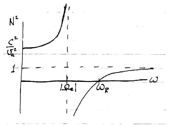
This is always above | Ωe |.
Figure 5.5:
The form of the dispersion relation for RH wave.
One can similarly investigate Left-hand wave and perpendicularly
propagating waves. The resulting wave resonances and cut-offs depend
only upon 2 properties (for specified ion mass) (1) Density
↔ ωpe2 (2) Magnetic Field
↔ | Ωe |. [Ion values ωpi,
| Ωi | are got by [(mi)/(me)] factors.]
These resonances and cutoffs are often plotted on a 2-D plane
[( | Ωe |)/(ω)] , [(ωp2)/(ω2)] ( ∝ B, n) called the
C M A Diagram.
We don't have time for it here.
5.3.2 Hybrid Resonances Perpendicular Propagation
"Extraordinary" wave N2 = [R L/S]
Polarization Ez=0, [(Ey)/(Ex)] = [iDS/(RL −S2)]=[(−iS)/D],
because RL=S2−D2.
|
N2 = |
|
| ⎡
⎣
|
( ω+ Ωe ) ( ω+ Ωi ) − |
ωpe2
ω
|
( ω+ Ωi ) − |
ωpi2
ω
|
( ω+ Ωe ) | ⎤
⎦
|
| ⎡
⎣
|
( ω− Ωe ) ( ω− Ωi ) − |
ωpe2
ω
|
( ω− Ωi )... | ⎤
⎦
|
|
( ω2 − Ωe2 ) ( ω2 − Ωi2) − ωpe2 ( ω2 − Ωi2 ) − ωpi2 ( ω2 − Ωe2 )
|
|
| (5.88) |
Resonance is where denominator = 0.
Solve the quadratic in ω2 and one gets
| |
|
|
|
1
2
|
| ⎡
⎣
|
( ωpe2 + Ωe2 + ωpi2 + Ωi2) |
| |
| |
|
|
± |
√
|
( ωpe2 + Ωe2 + ωpi2 + Ωi2)2 −4(Ωe2Ωi2+ωpe2Ωi2+ωpi2Ωe2)
|
| ⎤
⎦
|
|
| | (5.89) |
| |
|
|
ωpe2 + Ωe2 + ωpi2 + Ωi2
2
|
± |
⎛
√
|
|
| ⎛
⎝
|
ωpe2 + Ωe2 − ωpi2 − Ωi2
2
| ⎞
⎠
|
2
|
+ ωpe2 ωpi2 |
|
|
| | (5.90) |
|
Neglecting terms of order [(me)/(mi)] (e.g.
[(ωpi2)/(ωpe2)]) one gets
solutions
| |
|
|
ωpe2 + Ωe2 Upper Hybrid Resonance. |
| | (5.91) |
| |
|
|
Ωe2 ωpi2
Ωe2 + ωpe2
|
Lower Hybrid Resonance.. |
| | (5.92) |
|
At very high density,
ωpe2 >> Ωe2
geometric mean of cyclotron frequencies.
At very low density, ωpe2 << Ωe2
ion plasma frequency
Usually in tokamaks ωpe2 ∼ Ωe2.
Intermediate.
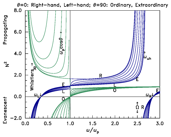
Summary Graph (Ω > ωp)
Figure 5.6: Summary of magnetized dispersion
relation for different propagation angles.
Cut-offs are where N2 = 0.
Resonances are where N2 → ∞.
Intermediate angles of propagation have refractive indices
between the θ = 0, [(π)/2] lines, in the
shaded areas.
5.3.3 Whistlers
(Ref. R.A. Helliwell, "Whistlers & Related Ionospheric
Phenomena," Stanford UP 1965.)
For N2 >> 1 the right hand wave can be written
|
N2 ≅ |
− ωpe2
ω( ω− | Ωe | )
|
, (N = kc/ω) |
| (5.95) |
Group velocity is
|
vg = |
d ω
dk
|
= | ⎛
⎝
|
dk
dω
| ⎞
⎠
|
−1
|
= | ⎡
⎣
|
d
dω
|
| ⎛
⎝
|
Nω
c
| ⎞
⎠
| ⎤
⎦
|
−1
|
. |
| (5.96) |
Then since
|
N = |
ωp
ω1/2 ( | Ωe | − ω)1/2
|
, |
| (5.97) |
we have
| |
|
|
|
d
d ω
|
|
ωp ω1/2
( | Ωe | − ω)1/2
|
= ωp | ⎧
⎨
⎩
|
ω1/2 (| Ωe | − ω)1/2
|
+ |
( | Ωe | − ω)3/2
| ⎫
⎬
⎭
|
|
| |
| |
|
|
|
ωp/2
( | Ωe | − ω)3/2 ω1/2
|
{( | Ωe | − ω) + ω} |
| |
| |
|
|
ωp | Ωe |/2
( | Ωe | − ω)3/2 ω1/2
|
|
| | (5.98) |
|
Thus
|
vg = |
c 2 ( | Ωe | − ω)3/2 ω1/2
ωp | Ωe |
|
|
| (5.99) |
Group Delay is
|
|
L
vg
|
∝ |
1
ω1/2 ( | Ωe | − ω)3/2
|
∝ |
1
|
| ⎛
⎝
|
ω
| Ωe |
| ⎞
⎠
|
1/2
|
| ⎛
⎝
|
1 − |
ω
| Ωe |
| ⎞
⎠
|
3/2
|
|
|
| (5.100) |
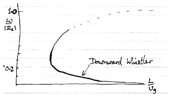
Figure 5.7: Whistler plot of frequency versus delay.
Plot with [ L/(vg)] as x-axis.
Resulting form explains downward whistle.
Lightning strike ∼ δ-function excites all
frequencies.
Lower ones arrive later.
Examples of actual whistler sounds can be obtained from
http://www-istp.gsfc.nasa.gov/istp/polar/polar_pwi_sounds.html.
5.4 Thermal Effects on Plasma Waves
The cold plasma approx is only good for high frequency,
N2 ∼ 1 waves. If ω is low or N2 >> 1 one may
have to consider thermal effects.
From the fluid viewpoint, this means pressure. Write
down the momentum equation. (We shall go back to
B0 = 0) linearized
|
mn |
∂v1
∂t
|
= n q E1 − ∇p1 ; |
| (5.101) |
remember these are the perturbations:
Fourier Analyse (drop 1's)
The key question: how to relate p to v
Answer: Equation of state + Continuity
State
|
p n−γ = const. ⇒ ( p0 + p1 ) ( n0 + n1 )−γ = p0 n0−γ |
| (5.104) |
Use Taylor Expansion
|
( p0 + p1 ) (n0 + n1 )−γ ≅ p0 n0−γ | ⎡
⎣
|
1 + |
p1
p0
|
− γ |
n1
n0
| ⎤
⎦
|
|
| (5.105) |
Hence
Continuity
Linearise:
|
|
∂n1
∂t
|
+ ∇ . (n0 v1 ) = 0 ⇒ |
∂n
∂t
|
+ n0 ∇ . v
= 0 |
| (5.108) |
Fourier Transform
|
− i ωn1 + n0 i k . v1 = 0 |
| (5.109) |
i.e.
Combine State & Continuity
|
p1 = p0 γ |
n1
n0
|
= p0 γ |
n0
|
= p0 γ |
k . v
ω
|
|
| (5.111) |
Hence Momentum becomes
|
m n0 ( −i ω) v= n q E− |
i k p0 γ
ω
|
k . v |
| (5.112) |
Notice Transverse waves have k . v
= 0; so they
are unaffected by pressure.
Therefore we need only consider the longitudinal wave.
However, for consistency let us proceed as before to get the
dielectric tensor etc.
Choose axes such that k = k ∧ez
then obviously:
|
vx = |
i q
ωm
|
Ex vy = |
i q
ωm
|
Ey |
| (5.113) |
|
vz = |
q
m
|
|
Ez
− i ω+ ( i k2 γp0 / m n0 ω)
|
|
| (5.114) |
Recall that p0=n0T so write p0/n0=T.
Then
|
σ = |
i n q2
ωm
|
| ⎡
⎢
⎢
⎢
⎢
⎢
⎢
⎣
|
|
| ⎤
⎥
⎥
⎥
⎥
⎥
⎥
⎦
|
|
| (5.115) |
|
ϵ = 1 + |
iσ
ϵ0 ω
|
= | ⎡
⎢
⎢
⎢
⎢
⎢
⎢
⎢
⎢
⎢
⎣
|
| ⎤
⎥
⎥
⎥
⎥
⎥
⎥
⎥
⎥
⎥
⎦
|
|
| (5.116) |
(Taking account only of 1 species, electrons, for now.)
We have confirmed the previous comment that the transverse
waves (Ex, Ey) are unaffected. The longitudinal
wave is. Notice that ϵ now
depends on k as well as ω. This is called
`spatial dispersion'.
For completeness, note that the dielectric tensor can be
expressed in general tensor notation as
| |
|
|
1 − |
ωp2
ω2
|
| ⎛
⎜
⎝
|
1 + k k | ⎡
⎢
⎣
|
1
|
− 1 | ⎤
⎥
⎦
| ⎞
⎟
⎠
|
|
| |
| |
|
| 1 − |
ωp2
ω2
|
| ⎛
⎜
⎝
|
1 + k k |
1
| ⎞
⎟
⎠
|
|
| | (5.117) |
|
This form shows isotropy with respect to the medium: there
is no preferred direction in space for the wave vector
k.
But once k is chosen, ϵ is not isotropic.
The direction of k becomes a special direction.
Longitudinal Waves: dispersion relation is
which is
or
|
ω2 = ωp2 + k2 |
γT
m
|
= ωp2 + k2 γvt2 . |
| (5.120) |
[The appropriate value of γ to take is 1 dimensional
adiabatic i.e. γ = 3. This seems plausible since
the electron motion is 1-d (along k) and may be demonstrated
more rigorously by kinetic theory.]
The above dispersion relation is called the Bohm-Gross
formula for electron plasma waves. Notice the group
velocity:
|
vg = |
dω
dk
|
= |
1
2ω
|
|
d ω2
dk
|
= |
γk vt2
( ωp2 + γk2 vt2 )1/2
|
≠ 0. |
| (5.121) |
and for kvt > ωp this tends to γ1/2 vt.
In this limit energy travels at the electron thermal speed.
5.4.1 Refractive Index Plot
Bohm Gross electron plasma waves:
|
N2 = |
c2
γe vte2
|
| ⎛
⎝
|
1 − |
ωp2
ω2
| ⎞
⎠
|
|
| (5.122) |
Transverse electromagnetic waves:
These have just the same shape except the electron plasma
waves have much larger vertical scale:
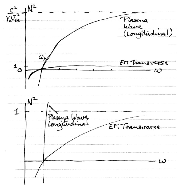
Figure 5.8: Refractive Index Plot. Top plot on the
scale of the Bohm-Gross Plasma waves. Bottom plot, on the scale of the
E-M transverse waves
On the E-M wave scale, the plasma wave curve is nearly vertical.
In the cold plasma it was exactly
vertical.
We have relaxed the Cold Plasma approximation.
5.4.2 Including the ion response
As an example of the different things which can
occur when ions are allowed to move, include longitudinal
ion response:
|
0 = ϵzz = 1 − |
ωpe2
|
− |
ωpi2
|
|
| (5.124) |
This is now a quadratic equation for ω2 so there
are two ω solutions possible for a given k. One
will be in the vicinity of the electron plasma wave
solution and the inclusion of ωpi2 which is
<< ωpe2 will give a small correction.
Second solution will be where the third term is same
magnitude as second (both will be >> 1). This will be
at low frequency. So we may write the dispersion relation
approximately as:
i.e.
| |
|
|
k2γi Ti
mi
|
+ |
ωpi2
ωpe2
|
|
k2 γe Te
me
|
= k2 | ⎡
⎣
|
γi Ti + γe Te
mi
| ⎤
⎦
|
|
| | (5.126) |
|
[In this case the electrons have time to stream through
the wave in 1 oscillation so they tend to be isothermal:
i.e. γe = 1. What to take for γi is less
clear, and less important because kinetic theory shows
that these waves we have just found are strongly damped
unless Ti << Te.]
These are `ion-acoustic' or `ion-sound' waves
cs is the sound speed
|
cs2 = |
γi Ti + Te
mi
|
≅ |
Te
mi
|
|
| (5.128) |
Approximately non-dispersive waves with phase velocity cs.
5.5 Electrostatic Approximation for (Plasma) Waves
The dispersion relation is written generally as
|
N ∧( N ∧E) + ϵ . E= N ( N . E) − N2 E+ ϵ . E= 0 |
| (5.129) |
Consider E to be expressible as longitudinal and transverse
components El, Et such that N ∧El = 0, N . Et = 0 . Then the
dispersion relation can be written
|
N ( N . El ) − N2 ( El + Et ) + ϵ . ( El + Et ) = − N2 Et + ϵ . Et + ϵ .El = 0 |
| (5.130) |
or
Now the electric field can always be written as the sum
of a curl-free component plus a divergenceless component,
e.g. conventionally
|
E= |
− ∇ϕ
[(Curl−free) || Electrostatic]
|
+ |
[(Divergence−free) || Electromagnetic]
|
|
| (5.132) |
and these may be termed electrostatic and electromagnetic
parts of the field.
For a plane wave, these two parts are clearly the same as the
longitudinal and transverse parts because
|
− ∇ϕ = − i k ϕ is longitudinal |
| (5.133) |
and if ∇ . · A = 0 (because
∇ . A = 0 (w.l.o.g.))
then k . · A = 0 so · A is
transverse.
`Electrostatic' waves are those that are describable
by the electrostatic part of the electric field, which is the
longitudinal part: | El | >> | Et |.
If we simply say Et = 0 then the dispersion relation
becomes ϵ . El = 0. This is not
the most general dispersion relation for electrostatic waves. It
is too restrictive. In general, there is a more significant
way in which to get solutions where
| El | >> | Et |. It is for N2 to be
very large compared to all the components of ϵ :N2 >> ||ϵ||.
If this is the case, then the dispersion relation is
approximately
Et is small but not zero.
We can then annihilate the Et term by taking the N
component of this equation; leaving
|
N . ϵ . El = 0 or ( N . ϵ . N ) El = 0 : k . ϵ . k = 0 . |
| (5.135) |
When the medium is isotropic there is no relevant difference
between the electrostatic dispersion relation:
and the purely longitudinal case ϵ . N = 0.
If we choose axes such that N is along ∧z, then
the medium's isotropy ensures the off-diagonal components of
ϵ are zero so N . ϵ . N = 0
requires ϵzz = 0 ⇒ ϵ . N = 0.
However if the medium is not isotropic, then even if
|
N . ϵ . N ( = N2 ϵzz ) = 0 |
| (5.137) |
there may be off-diagonal terms of ϵ that make
In other words, in an anisotropic medium (for example a
magnetized plasma) the electrostatic approximation can give
waves that have non-zero transverse electric field (of order
||ϵ|| / N2 times El) even though
the waves are describable in terms of a scalar potential.
To approach this more directly, from Maxwell's equations, applied
to a dielectric medium of dielectric tensor ϵ,
the electrostatic part of the electric field is derived from
the electric displacement
|
∇ . D = ∇ . ( ϵ0 ϵ . E) = ρ = 0 (no free charges) |
| (5.139) |
So for plane waves 0 = k . D = k . ϵ . E
= i k . ϵ . k ϕ.
The electric displacement, D, is purely transverse (not
zero) but the electric field, E then gives rise to an
electromagnetic
field via ∇ ∧H = ∂D/∂t.
If N2 >> ||ϵ|| then this magnetic
(inductive) component can be considered as a benign passive
coupling to the electrostatic wave.
In summary, the electrostatic dispersion relation is k. ϵ . k=0, or in coordinates where
k is in the z-direction, ϵzz=0.
5.6 Simple Example of MHD Dynamics: Alfven Waves
Ignore Pressure & Resistivity.
Linearize:
|
V = V1, B
= B0 + B1 (B0 uniform), j
= j1. |
| (5.142) |
Fourier Transform:
Eliminate V by taking 5.145 ∧B0 and substituting
from 5.146.
|
E+ |
1
− i ωρ
|
( j∧B0 ) ∧B0 = 0 |
| (5.147) |
or
|
E= − |
1
− i ωρ
|
{ ( j. B0 ) B0 − B02 j} = |
B02
− i ωρ
|
j⊥ |
| (5.148) |
So conductivity tensor can be written (z in B direction).
|
σ = |
− i ωρ
B02
|
| ⎡
⎢
⎢
⎢
⎣
|
|
| ⎤
⎥
⎥
⎥
⎦
|
|
| (5.149) |
where ∞ implies that E|| = 0 (because of
Ohm's law). Hence Dielectric Tensor
|
ϵ = 1 + |
σ
− i ωϵ0
|
= | ⎛
⎝
|
1 + |
ρ
ϵ0 B2
| ⎞
⎠
|
| ⎡
⎢
⎢
⎢
⎣
|
|
| ⎤
⎥
⎥
⎥
⎦
|
. |
| (5.150) |
Dispersion tensor in general is:
|
K= |
ω2
c2
|
[ N N − N2 + ϵ ] |
| (5.151) |
Dispersion Relation taking N⊥ = Nx, Ny=0
|
|K|= | ⎢
⎢
⎢
⎢
⎢
⎢
⎢
⎢
|
|
| ⎢
⎢
⎢
⎢
⎢
⎢
⎢
⎢
|
= 0 |
| (5.152) |
Meaning of ∞ is that the cofactor must be zero i.e.
|
| ⎛
⎝
|
− N||2 + 1 + |
ρ
ϵ0 B2
| ⎞
⎠
|
| ⎛
⎝
|
− N2 + 1 + |
ρ
ϵ0 B2
| ⎞
⎠
|
= 0 |
| (5.153) |
The 1's here come from Maxwell displacement current and are usually
negligible (N⊥2 >> 1). So final waves are
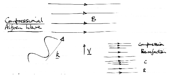
Figure 5.9:
Compressional Alfven Wave. Works by magnetic pressure (primarily).
- N2 = [(ρ)/(ϵ0 B2)] ⇒ Non-dispersive
wave with phase and group velocities
|
vp = vg = |
c
N
|
= | ⎛
⎝
|
c2 ϵ0 B2
ρ
| ⎞
⎠
|
1/2
|
= | ⎡
⎣
|
B2
μ0 ρ
| ⎤
⎦
|
1/2
|
|
| (5.154) |
where we call
|
| ⎡
⎣
|
B2
μ0 ρ
| ⎤
⎦
|
1/2
|
≡ vA the `Alfven Speed′ |
| (5.155) |
Polarization:
|
E|| = Ez = 0, Ex = 0. Ey ≠ 0 ⇒ Vy = 0 Vx ≠ 0 (Vz = 0) |
| (5.156) |
Party longitudinal (velocity) wave → Compression
"Compressional Alfven Wave".
- N||2 = [( ρ)/(ϵ0 B2)] = [( k||2 c2)/(ω2)]
Any ω has unique k||. Wave has unique velocity
in || direction: vA.
Polarization
|
Ez = Ey = 0 Ex ≠ 0 ⇒ Vx = 0 Vy ≠ 0 (Vz = 0) |
| (5.157) |
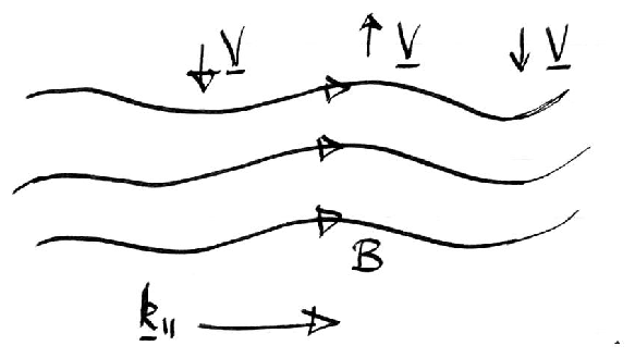
Transverse velocity: "Shear Alfven Wave".
Figure 5.10: Shear Alfven Wave
Works by field line bending (Tension Force) (no compression).
5.7 Non-Uniform Plasmas and wave propagation
Practical plasmas are not infinite & homogeneous. So
how does all this plane wave analysis apply practically?
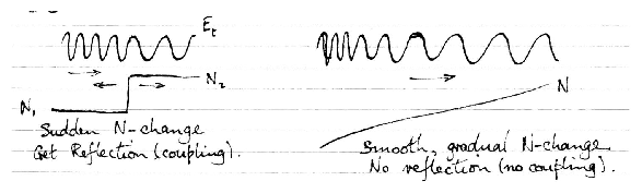
If the spatial variation of the plasma is slow c.f. the
wave length of the wave, then coupling to other waves will
be small (negligible).
Figure 5.11: Comparison of sudden and gradualy
refractive index change.
For a given ω, slowly varying plasma means
N/[dN/dx] >> λ or
k N/[dN/dx] >> 1. Locally, the plasma appears
uniform.
Even if the coupling is small, so that locally the wave propagates
as if in an infinite uniform plasma, we still need a way of
calculating how the solution propagates from one place to the
other. This is handled by the `WKB(J)' or `eikonal' or
`ray optic' or `geometric optics' approximation.
WKBJ solution
Consider the model 1-d wave equation (for field ω)
with k now a slowly varying function of x. Seek a solution
in the form
|
E = exp( i ϕ( x ) ) (− i ωt implied) |
| (5.159) |
ϕ is the wave phase ( = kx in uniform plasma).
Differentiate twice
|
|
d2 E
d x2
|
= { i |
d2 ϕ
d x2
|
− | ⎛
⎝
|
d ϕ
d x
| ⎞
⎠
|
2
|
} eiϕ |
| (5.160) |
Substitute into differential equation to obtain
|
| ⎛
⎝
|
d ϕ
d x
| ⎞
⎠
|
2
|
= k2 + i |
d2 ϕ
d x2
|
|
| (5.161) |
Recognize that in uniform plasma [(d2 ϕ)/(d x2)] = 0.
So in slightly non-uniform, 1st approx is to ignore this term.
Then obtain a second approximation by substituting
so
| |
|
| | (5.164) |
| |
|
| ± | ⎛
⎝
|
k ± |
i
2 k
|
|
d k
d x
| ⎞
⎠
|
using Taylor expansion. |
| | (5.165) |
|
Integrate:
|
ϕ ≅ ± | ⌠
⌡
|
x
|
k d x + i ln( k1/2 ) |
| (5.166) |
Hence E is
|
E = ei ϕ = |
1
k1/2
|
exp | ⎛
⎝
|
±i | ⌠
⌡
|
x
|
k d x | ⎞
⎠
|
|
| (5.167) |
This is classic WKBJ solution. Originally studied by
Green
& Liouville (1837), the Green of Green's functions, the Liouville of
Sturm Liouville theory.
Basic idea of this approach: (1) solve the local dispersion
relation as if in infinite homogeneous plasma, to get
k(x), (2) form approximate solution for all space as above.
Phase of wave varies as integral of k d x.
In addition, amplitude varies as [1/(k1/2 )].
This is required to make the total energy flow uniform.
5.8 Two Stream Instability
An example of waves becoming unstable in a non-equilibrium plasma.
Analysis is possible using Cold Plasma techniques.
Consider a plasma with two participating cold species but having
different average velocities.
These are two "streams".
We can look at them in different inertial frames, e.g.
species (stream) 2 stationary or 1 stationary (or neither).
We analyse by obtaining the susceptibility for each species
and adding together to get total dielectric constant (scalar
1-d if unmagnetized).
In a frame of reference in which it is stationary, a stream
j has the (Cold Plasma) susceptibility
If the stream is moving with velocity vj (zero order) then
its susceptibility is
|
χj = |
− ωpj2
( ω− k vj )2
|
. (k & vj in same direction) |
| (5.170) |
Proof from equation of motion:
|
|
qj
mj
|
E = |
∂t
|
+ v. ∇ |
~
v
|
= ( − i ω+ i k . vj ) |
~
v
|
= − i ( ω− k vj ) |
~
v
|
. |
| (5.171) |
Current density
|
jj = ρj vj + ρj . |
~
v
|
j
|
+ |
~
ρ
|
vj . |
| (5.172) |
Substitute in
| |
|
|
i k . |
~
v
|
ρ+ i k . |
~
v
|
ρ− i ω |
~
ρ
|
= 0 |
| | (5.173) |
| |
|
| | (5.174) |
|
Hence substituting for ~v in terms of E:
|
− χj ϵ0 ∇ . E= |
~
ρ
|
j
|
= |
ρj qj
mj
|
|
k . E
−i ( ω− k .vj )2
|
, |
| (5.175) |
which shows the longitudinal susceptibility is
|
χj = − |
ρj qj
mj ϵ0
|
|
1
( ω2 − k vj )2
|
= |
− ωpj2
( ω− k vj )2
|
|
| (5.176) |
Proof by transforming frame of reference:
Consider Galilean transformation to a frame moving with the
stream at velocity vj.
|
expi ( k . x− ωt ) = expi ( k . x′− ( ω− k .vj ) t′) |
| (5.178) |
So in frame of the stream, ω′ = ω− k . vj.
Substitute in stationary cold plasma expression:
|
χj = − |
ωpj2
ω′2
|
= − |
ωpj2
( ω− k vj )2
|
. |
| (5.179) |
Thus for n streams we have
|
ϵ = 1 + |
∑
j
|
χj = 1 − |
∑
j
|
|
ωpj2
( ω− k vj )2
|
. |
| (5.180) |
Longitudinal wave dispersion relation is
Two streams
|
0 = ϵ = 1 − |
ωp12
( ω− k v1 )2
|
− |
ωp22
( ω− k v2 )2
|
|
| (5.182) |
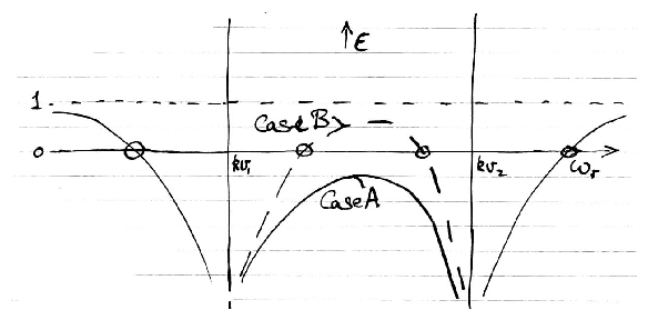
For given real k this is a quartic in ω. It has
the form:
Figure 5.12: Two-stream stability analysis.
If ϵ crosses zero between the wells, then
∃ 4 real solutions for ω. (Case B).
If not, then 2 of the solutions are complex:
ω = ωr ±i ωi (Case A).
The time dependence of these complex roots is
|
exp(−i ωt ) = exp( − i ωr t ±ωi t ) . |
| (5.183) |
The +ve sign is growing in time: instability.
It is straightforward to show that Case A occurs if
|
| k (v2 − v1) | < [ ωp12/3 + ωp22/3 ]3/2 . |
| (5.184) |
Small enough k (long enough wavelength) is always unstable.
Simple interpretation (ωp22 << ωp12,
v1 = 0) a tenuous beam in a plasma sees a negative ϵ
if | k v2 | < ∼ ωp1 .
Negative ϵ implies charge perturbation causes E
that enhances itself: charge (spontaneous) bunching.
5.9 Kinetic Theory of Plasma Waves
Wave damping is due to wave-particle resonance. To treat this
we need to keep track of the particle distribution in velocity
space → kinetic theory.
5.9.1 Vlasov Equation
Treat particles as moving in 6-D phase space x position,
v velocity. At any instant a particle occupies a unique
position in phase space (x,v).
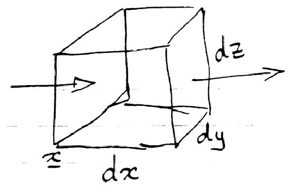
Consider an elemental volume d3 xd3 v of phase space
[dx dy dz dvx dvy dvz], at (x, v). Write down
an equation that is conservation of particles for this
volume
| |
|
|
| ⎡
⎣
|
vx f | ⎛
⎝
|
x+ d x |
^
x
|
, v | ⎞
⎠
|
− vx f ( x, v) | ⎤
⎦
|
dy dz d3 v |
| |
| |
|
| |
| |
|
|
| ⎡
⎣
|
ax f | ⎛
⎝
|
x, v+ d vx |
^
x
| ⎞
⎠
|
−ax f ( x, v) | ⎤
⎦
|
d3 xd vy d vz |
| |
| |
|
| | (5.185) |
|
Figure 5.13: Difference in flow across x-surfaces (+y+z).
a is "velocity space motion", i.e. acceleration.
Divide through by d3 xd3 v and take limit
| |
|
|
|
∂
∂x
|
( vx f ) + |
∂
∂y
|
( vy f ) + |
∂
∂z
|
( vz f ) + |
∂
∂vx
|
( ax f ) + |
∂
∂vy
|
( ay f ) + |
∂
∂vz
|
( az f ) |
| |
| |
|
| ∇ . ( vf ) + ∇v . ( a f ) |
| | (5.186) |
|
[Notation: Use [(∂)/(∂x)] ↔ ∇ ; [(∂)/(∂v)] ↔ ∇v ].
Take this simple continuity equation in phase space and expand:
|
|
∂f
∂t
|
+ ( ∇ . v)f + ( v. ∇ ) f + ( ∇v .a ) f + ( a . ∇v ) f = 0 . |
| (5.187) |
Recognize that ∇ means here [(∂)/(∂x)]
etc. keeping v constant so that
∇ . v
= 0 by definition. So
|
|
∂f
∂t
|
+ v. |
∂f
∂x
|
+ a . |
∂f
∂v
|
= − f ( ∇v . a ) |
| (5.188) |
Now we want to couple this equation with Maxwell's equations
for the fields, and the Lorentz force
Actually we don't want to use the E retaining all the local
effects of individual particles. We want a smoothed out field.
Ensemble averaged E.
Evaluate
| |
|
|
∇v . |
q
m
|
( E+ v∧B) = |
q
m
|
∇v . ( v∧B) |
| | (5.190) |
| |
|
| | (5.191) |
|
So RHS is zero. However in the use of smoothed out E we have
ignored local effect of one particle on another due to the
graininess. That is collisions.
Boltzmann Equation:
|
|
∂f
∂t
|
+ v. |
∂f
∂x
|
+ a . |
∂f
∂v
|
= | ⎛
⎝
|
∂f
∂t
| ⎞
⎠
|
collisions
|
|
| (5.192) |
Vlasov Equation ≡ Boltzman Eq without collisions.
For electromagnetic forces:
|
|
∂f
∂t
|
+ v. |
∂f
∂x
|
+ |
q
m
|
( E+ v∧B) |
∂f
∂v
|
= 0 . |
| (5.193) |
Interpretation:
Distribution function is constant along particle orbit in phase
space: [d/dt] f = 0.
|
|
d
dt
|
f = |
∂f
∂t
|
+ |
d x
d t
|
. |
∂f
∂x
|
+ |
∂v
d t
|
. |
∂f
∂v
|
|
| (5.194) |
Coupled to Vlasov equation for each particle species we have
Maxwell's equations.
Vlasov-Maxwell Equations
| |
|
|
v. |
∂fj
∂x
|
+ |
qj
mj
|
( E+ v∧B) . |
∂fj
∂vj
|
= 0 |
| | (5.195) |
| |
|
|
|
− ∂B
∂t
|
, ∇ ∧B
= μ0 j+ |
1
c2
|
|
∂E
∂t
|
|
| | (5.196) |
| |
|
| | (5.197) |
|
Coupling is completed via charge & current densities.
| |
|
|
|
∑
j
|
qj nj = |
∑
J
|
qj | ⌠
⌡
|
fj d3v |
| | (5.198) |
| |
|
|
∑
j
|
qj nj Vj = |
∑
j
|
qj | ⌠
⌡
|
fj vd3 v. |
| | (5.199) |
|
Describe phenomena in which collisions are not important,
keeping track of the (statistically averaged) particle
distribution function.
Plasma waves are the most important phenomena covered by
the Vlasov-Maxwell equations.
6-dimensional, nonlinear, time-dependent, integral-differential
equations!
5.9.2 Linearized Wave Solution of Vlasov Equation
Unmagnetized Plasma
Linearize the Vlasov Eq by supposing
| |
|
|
f0 (v) + f1 (v) expi ( k . x− ωt ) , f1 small. |
| | (5.200) |
| |
|
| E1 expi ( k . x− ωt) B
= B1 expi ( k . x− ωt ) |
| | (5.201) |
|
Zeroth order f0 equation satisfied by
[(∂)/(∂t)] , [(∂)/(∂x)] = 0.
First order:
|
− i ωf1 + v. i k f1 + |
q
m
|
( E1 +v∧B1 ) . |
∂f0
∂v
|
= 0 . |
| (5.202) |
[Note v is not per se of any order, it is an independent
variable.]
Solution:
|
f1 = |
1
i ( ω− k . v)
|
|
q
m
|
( E1 + v∧B1 ) . |
∂f0
∂v
|
|
| (5.203) |
For convenience, assume f0 is isotropic. Then
[(∂f0)/(∂v)] is in direction
v so v∧B1 . [(∂f0)/(∂v)] = 0
We want to calculate the conductivity σ.
Do this by simply integrating:
|
j= | ⌠
⌡
|
q f1 vd3 v = |
q2
i m
|
| ⌠
⌡
|
|
ω− k . v
|
d3 v . E1. |
| (5.205) |
Here the electric field has been taken outside the v-integral but
its dot product is with ∂f0/∂v.
Hence we have the tensor conductivity,
|
σ = |
q2
i m
|
| ⌠
⌡
|
|
ω− k . v
|
d3 v |
| (5.206) |
Focus on zz component:
|
1 + χzz = ϵzz = 1 + |
σzz
− i ωϵ0
|
= 1 + |
q2
ωm ϵ0
|
| ⌠
⌡
|
|
ω− k . v
|
d3 v |
| (5.207) |
Such an expression applies for the conductivity
(susceptibility) of each species, if more than one
needs to be considered.
It looks as if we are there! Just do the integral!
Now the problem becomes evident. The integrand has a zero
in the denominator. At least we can do 2 of 3 integrals
by defining the 1-dimensional distribution function
|
fz (vz) ≡ | ⌠
⌡
|
f (v) d vx d vy (k = k |
^
z
|
) |
| (5.208) |
Then
|
χ = |
q2
ωm ϵ0
|
| ⌠
⌡
|
|
ω− k vz
|
d vz |
| (5.209) |
(drop the z suffix from now on. 1-d problem).
How do we integrate through the pole at v = [( ω)/k]?
Contribution of resonant particles. Crucial to get right.
Path of velocity integration
First, realize that the solution we have found is not complete.
In fact a more general solution can be constructed by adding
any solution of
[We are dealing with 1-d Vlasov equation:
[(∂f)/(∂t)] + v [(∂f)/(∂z)] + [q E/m] [(∂f)/(∂v)] = 0.]
Solution of this is
where g is an arbitrary function of its arguments. Hence
general solution is
|
f1 = |
i ( ω− k v )
|
expi ( k z − ωt ) + g ( v t − z, v ) |
| (5.212) |
and g must be determined by initial conditions. In general,
if we start up the wave suddenly there will be a transient
that makes g non-zero.
So instead we consider a case of complex ω (real k for
simplicity) where ω = ωr + i ωi and ωi > 0.
This case corresponds to a growing wave:
|
exp( − i ωt ) = exp( − i ωr t + ωi t ) |
| (5.213) |
Then we can take our initial condition to be f1=0 at t → −∞. This is satisfied by taking g = 0.
For ωi > 0 the complementary function, g, is zero.
Physically this can be thought of as treating a case where there is a
very gradual, smooth start up, so that no transients are generated.
Thus if ωi > 0, the solution is simply the velocity integral,
taken along the real axis, with no additional terms.
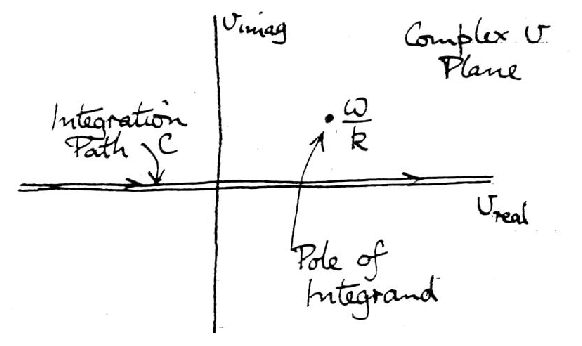
For
|
ωi > 0, χ = |
q2
ωm ϵ0
|
| ⌠
⌡
|
C
|
|
ω− k v
|
d v |
| (5.214) |
where there is now no difficulty about the integration because
ω is complex.
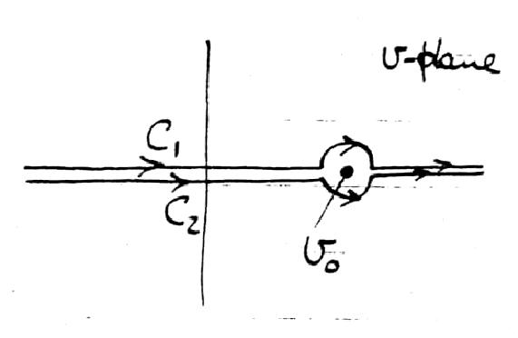
Figure 5.14: Contour of integration in complex v-plane.
The pole of the integrand is at v = [(ω)/k]
which is above the real axis.
The question then arises as to how to do the calculation if
ωi ≤ 0. The answer is by "analytic continuation",
regarding all quantities as complex.
"Analytic Continuation" of χ is accomplished by
allowing ω/k to move (e.g. changing the ωi) but
never allowing any poles to cross the integration contour, as
things change continuously.
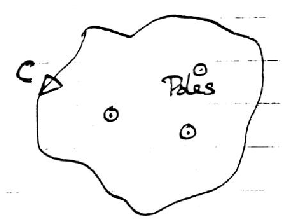
Remember (Fig 5.15)
|
| ⌠
(⎜)
⌡
|
c
|
F d z = |
∑
| residues ×2 πi |
| (5.215) |
(Cauchy's theorem)
Figure 5.15: Cauchy's theorem.
Where residues = limz→ zk[F(z)/(z−zk)] at the
poles, zk, of F(z). We can deform the contour
how we like, provided no poles cross it.
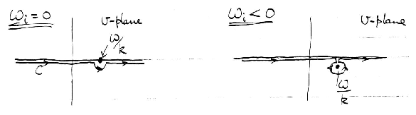
Hence contour (Fig 5.16)
Figure 5.16: Landau Contour
We conclude that the integration contour for ωi < 0 is
not just along the real v axis. It includes the pole
also.
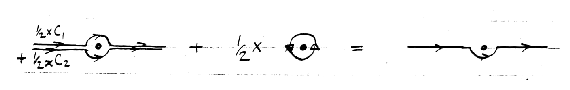
To express our answer in a universal way we use the
notation of "Principal Value" of a singular integral
defined as the average of paths above and below
|
℘ | ⌠
⌡
|
|
F
v − v0
|
d v = |
1
2
|
| ⎡
⎣
| ⌠
⌡
|
C1
|
+ | ⌠
⌡
|
C2
| ⎤
⎦
|
|
F
v − v0
|
d v |
| (5.216) |
Figure 5.17: Two halves of principal value contour.
Then
|
χ = |
q2
ωm ϵ0
|
{ ℘ | ⌠
⌡
|
|
ω− k v
|
d v − |
1
2
|
2 πi |
ω
k2
|
|
∂f0
∂v
| ⎢
⎢
|
v = [(ω)/k]
|
} |
| (5.217) |
Second term is half the normal residue term; so it is half of the
integral round the pole.
Figure 5.18: Contour equivalence.
Our expression is only short-hand for the (Landau) prescription:
|
"Integrate below the pole".
(Nautilus). |
Contribution from the pole can be considered to arise from the
complementary function g(v t − z, v). If g is to be
proportional to exp(ikz), then it must be of the form
g = exp[i k (z − vt)] h(v) where h(v)
is an arbitrary function. To get the result previously
calculated, the value of h(v) must be (for real ω)
|
h(v) = Eπ |
q
m
|
|
1
k
|
|
∂f0
∂v
| ⎢
⎢
|
w/k
|
δ | ⎛
⎝
|
v − |
ω
k
| ⎞
⎠
|
|
| (5.218) |
|
(so that | ⌠
⌡
|
|
q
− i ωϵ0
|
v g d v = |
q2
ωm ϵ0
|
| ⎛
⎝
|
πi |
ω
k2
|
|
∂f0
∂v
| ⎢
⎢
|
[(ω)/k]
| ⎞
⎠
|
. ) |
| (5.219) |
This Dirac delta function says that the complementary function
is limited to particles with "exactly" the wave phase
speed [(ω)/k]. It is the resonant behaviour of
these particles and the imaginary term they contribute to
χ that is responsible for wave damping or growth.
We shall see in a moment, that the standard case will be
ωi < 0, so the opposite of the prescription
ωi > 0 that makes g = 0. Therefore there will
generally be a complementary function, non-zero, describing
resonant effects. We don't have to calculate it explicitly
because the Landau prescription takes care of it.
5.9.3 Landau's original approach. (1946)
Corrected Vlasov's assumption that the correct result was just
the principal value of the integral. Landau recognized the
importance of initial conditions and so used Laplace Transform
approach to the problem
|
|
~
A
|
(p) = | ⌠
⌡
|
∞
0
|
e−pt A(t) dt |
| (5.220) |
The Laplace Transform inversion formula is
|
A(t) = |
1
2 πi
|
| ⌠
⌡
|
s+i∞
s−i∞
|
ept |
~
A
|
(p) dp |
| (5.221) |
where the path of integration must be chosen to the right of any
poles of ~A(p) (i.e. s large enough). Such a
prescription seems reasonable. If we make ℜ(p) large enough
then the ~A(p) integral will presumably exist. The
inversion formula can also be proved rigorously so that gives
confidence that this is the right approach.
If we identify p → − i ω, then the transform is
~A = ∫ei ωt A(t) dt, which can be identified as
the Fourier transform that would give component ~A ∝ e−i ωt, the wave we are discussing. Making ℜ(p)
positive enough to be to the right of all poles is then equivalent to
making ℑ(ω) positive enough so that the path in ω-space is
above all poles, in particular ωi > ℑ(kv). For real velocity, v,
this is precisely the condition ωi > 0, we adopted before to justify putting
the complementary function zero.
Either approach gives the same prescription. It is all bound up
with satisfying causality.
5.9.4 Solution of Dispersion Relation
We have the dielectric tensor
|
ϵ = 1 + χ = 1 + |
q2
ωm ϵ0
|
| ⎧
⎨
⎩
|
℘ | ⌠
⌡
|
|
ω− k v
|
d v − πi |
ω
k2
|
|
∂f0
∂v
| ⎢
⎢
|
[(ω)/k]
| ⎫
⎬
⎭
|
, |
| (5.222) |
for a general isotropic distribution. We also know that
the dispersion relation is
|
| ⎡
⎢
⎢
⎢
⎣
|
|
| ⎤
⎥
⎥
⎥
⎦
|
= ( −N2 + ϵt )2 ϵ = 0 |
| (5.223) |
Giving transverse waves N2 = ϵt and
longitudinal waves ϵ = 0. We need to do the integral and hence get ϵ.
Presumably, if we have done this right, we ought to be able to
get back the cold-plasma result as an approximation in the
appropriate limits, plus some corrections. We previously
argued that cold-plasma is valid if [(ω)/k] >> vt.
So regard [kv/(ω)] as a small quantity and expand:
| |
|
|
|
1
ω
|
| ⌠
⌡
|
v |
∂f0
∂v
|
| ⎡
⎣
|
1 + |
kv
ω
|
+ | ⎛
⎝
|
kv
ω
| ⎞
⎠
|
2
|
+ ... | ⎤
⎦
|
dv |
| |
| |
|
|
|
−1
ω
|
| ⌠
⌡
|
f0 | ⎡
⎣
|
1 + |
2 kv
ω
|
+ 3 | ⎛
⎝
|
kv
ω
| ⎞
⎠
|
2
|
+ ... | ⎤
⎦
|
dv (by parts) |
| |
| |
|
|
− 1
ω
|
| ⎡
⎣
|
n + |
3 n T
m
|
|
k2
ω2
| ⎤
⎦
|
+ ... |
| | (5.224) |
|
Here we have assumed we are in the particles' average rest frame
(no bulk velocity) so that ∫f0 vdv = 0 and also we have used
the temperature definition
appropriate to one degree of freedom (1-d problem).
Ignoring the higher order terms we get:
|
ϵ = 1 − |
ωp2
ω2
|
| ⎧
⎨
⎩
|
1 + 3 |
T
m
|
|
k2
ω2
|
+ πi |
ω2
k2
|
|
1
n
|
|
∂f0
∂v
| ⎢
⎢
|
[(ω)/k]
| ⎫
⎬
⎭
|
|
| (5.226) |
This is just what we expected. Cold plasma value was
ϵ = 1 − [(ωp2)/(ω2)]. We have
two corrections
- To real part of ϵ, correction 3 T/m[(k2)/(ω2)] = 3 ( [(vt)/(vp)] )2
due to finite temperature. We could have got this from a
fluid treatment with pressure.
- Imaginary part → antihermitian part of
ϵ→ dissipation.
Solve the dispersion relation for longitudinal waves
ϵ = 0 (again assuming k real ω complex).
Assume ωi << ωr then
| |
|
|
ωr2 + 2 ωr ωi i = ωp2 | ⎧
⎨
⎩
|
1 + 3 |
T
m
|
|
k2
ω2
|
+ πi |
ω2
k2
|
|
1
n
|
|
∂f0
∂v
| ⎢
⎢
|
[(ω)/k]
| ⎫
⎬
⎭
|
|
| |
| |
|
| ωp2 | ⎧
⎨
⎩
|
1 + 3 |
T
m
|
|
k2
ωr2
|
+ πi |
ωr2
k2
|
|
1
n
|
|
∂f0
∂v
| ⎢
⎢
|
[(ωr)/k]
| ⎫
⎬
⎭
|
|
| | (5.227) |
|
Hence
|
ωi ≅ |
1
2 ωr i
|
ωp2 πi |
ωr2
k2
|
|
1
n
|
|
∂f0
∂v
| ⎢
⎢
|
[(ωr)/k]
|
=ωp2 |
π
2
|
|
ωr
k2
|
|
1
n
|
|
∂f0
∂v
| ⎢
⎢
|
[(ωr)/k]
|
|
| (5.228) |
For a Maxwellian distribution
|
f0 = | ⎛
⎝
|
m
2 πT
| ⎞
⎠
|
1/2
|
exp | ⎛
⎝
|
− |
m v2
2 T
| ⎞
⎠
|
n |
| (5.229) |
|
|
∂f0
∂v
|
= | ⎛
⎝
|
m
2 πT
| ⎞
⎠
|
1/2
|
| ⎛
⎝
|
− |
m v
T
| ⎞
⎠
|
exp | ⎛
⎝
|
− |
m v2
2T
| ⎞
⎠
|
n . |
| (5.230) |
So, substituting,
|
ωi ≅ − ωp2 |
π
2
|
|
ωr2
k3
|
| ⎛
⎝
|
m
2 πT
| ⎞
⎠
|
1/2
|
|
m
T
|
exp | ⎛
⎝
|
− |
m ωr2
2 T k2
| ⎞
⎠
|
. |
| (5.231) |
The difference between ωr and ωp may not be
important in the outside but ought to be retained inside the
exponential since
|
|
m
2T
|
|
ωp2
k2
|
| ⎡
⎣
|
1 + 3 |
T
m
|
|
k2
ωp2
| ⎤
⎦
|
= |
m ωp2
2 T k2
|
+ |
3
2
|
. |
| (5.232) |
So
|
ωi ≅ − ωp | ⎛
⎝
|
π
8
| ⎞
⎠
|
1/2
|
|
ωp3
k3
|
|
1
vt3
|
exp | ⎛
⎝
|
− |
m ωp2
2 T k2
|
− |
3
2
| ⎞
⎠
|
. |
| (5.233) |
Imaginary part of ω is negative ⇒ damping.
This is Landau Damping.
Note that we have been treating a single species (electrons
by implication) but if we need more than one we simply add to
χ. Solution is then more complex.
5.9.5 Direct Calculation of Collisionless Particle Heating
(Landau Damping without complex variables!)
We show by a direct calculation that net energy is transferred
to electrons.
Suppose there exists a longitudinal wave
Equations of motion of a particle
Solve these assuming E is small by a perturbation expansion
v = v0 + v1 + ..., z = z0(t) + z1(t) + ... .
Zeroth order:
|
|
d v0
d t
|
= 0 ⇒ v0 = const , z0 = zi + v0 t |
| (5.237) |
where zi = const is the initial position.
First Order
| |
|
|
|
q
m
|
E cos( k z0 − ωt ) = |
q
m
|
E cos( k ( zi + v0 t ) − ωt ) |
| | (5.238) |
| |
|
| | (5.239) |
|
Integrate:
|
v1 = |
q E
m
|
|
sin( k zi + [k v0 − ω] t )
k v0 − ω
|
+ const. |
| (5.240) |
take initial conditions to be v1, v2 = 0.
Then
|
v1 = |
q E
m
|
|
sin( k zi + ∆ωt ) − sin( k zi )
∆ω
|
|
| (5.241) |
where ∆ω ≡ k v0 − ω, is (-) the
frequency at which the particle feels the wave field.
|
z1 = |
q E
m
|
| ⎡
⎣
|
cosk zi − cos( k zi + ∆ωt )
∆ω2
|
− t |
sink zi
∆ω
| ⎤
⎦
|
|
| (5.242) |
(using z1(0) = 0).
2nd Order (Needed to get energy right)
| |
|
|
|
q E
m
|
{cos( k z0 − ωt + k z1 ) − cos( k z0t − ωt ) } |
| |
| |
|
|
|
q E
m
|
{ cos( k z0 − ωt)cos( k z1) −sin( k z0 − ωt)sin( k z1) − cos( k z0t − ωt ) } |
| |
| |
|
| − |
q E
m
|
k z1 sin( k zi + ∆ωt ) (k z1 << 1) |
| | (5.243) |
|
Now the gain in kinetic energy of the particle is
| |
|
|
|
1
2
|
m { ( v0 + v1 + v2 + ... )2 − v02 } |
| |
| |
|
|
1
2
|
m { 2 v0 v1 + v12 + 2 v0 v2 + higher order } |
| | (5.244) |
|
The total rate of increase of K.E. is the average
of the time derivative of this over space, i.e. over zi.
|
< |
d
d t
|
| ⎛
⎝
|
1
2
|
m v2 | ⎞
⎠
|
> = m < v0 |
d v1
d t
|
+ v1 |
d v1
d t
|
+v0 |
d v2
d t
|
> |
| (5.245) |
The zi average will cancel any component that simply oscillates with
zi, such as sinkzi or sin(kzi+∆ωt) cos(kzi+∆ωt) but not cos2 kzi or sin2 kzi.
| |
|
| | (5.246) |
| |
|
|
|
q2 E2
m2
|
< |
sin( k zi + ∆ωt ) − sink zi
∆ω
|
cos( k zi + ∆ωt ) > |
| |
| |
|
|
|
q2 E2
m2
|
< |
− sin( k zi + ∆ωt ) cos∆ωt + cos( k zi + ∆ωt )sin∆ωt
∆ω
|
cos( k zi + ∆ωt ) > |
| |
| |
|
|
|
q2 E2
m2
|
< |
sin∆ωt
∆ω
|
cos2 ( k zi + ∆ωt ) > = |
q2 E2
2m2
|
|
sin∆ωt
∆ω
|
|
| | (5.247) |
| |
|
|
|
− q2 E2
m2
|
k v0 < | ⎛
⎝
|
cosk zi − cos( k zi + ∆ωt )
∆ω2
|
− t |
sink zi
∆ω
| ⎞
⎠
|
sin( k zi + ∆ωt ) > |
| |
| |
|
|
|
− q2 E2
m2
|
k v0 < |
sin∆ωt
∆ω2
|
cos2kzi − t |
cos∆ωt
∆ω
|
sin2 k zi > |
| |
| |
|
|
q2 E2
m2
|
|
k v0
2
|
| ⎡
⎣
|
− |
sin∆ωt
∆ω2
|
+ t |
cos∆ωt
∆ω
| ⎤
⎦
|
. |
| | (5.248) |
|
Hence
| |
|
|
|
q2 E2
2 m
|
| ⎡
⎣
|
sin∆ωt
∆ω
|
− k v0 |
sin∆ωt
∆ω2
|
+ k v0 t |
cos∆ωt
∆ω
| ⎤
⎦
|
|
| |
| |
|
|
q2 E2
2 m
|
| ⎡
⎣
|
− ωsin∆ωt
∆ω2
|
+ |
ωt
∆ω
|
cos∆ωt + t cos∆ωt | ⎤
⎦
|
. |
| | (5.249) |
|
This is the space-averaged power into particles of a specific
velocity v0. We need to integrate over the distribution function.
A trick identify helps:
| |
|
|
|
ωt
∆ω
|
cos∆ωt + t cos∆ωt = |
∂
∂∆ω
|
| ⎛
⎝
|
ωsin∆ωt
∆ω
|
+ sin∆ωt | ⎞
⎠
|
|
| |
| |
|
|
1
k
|
|
∂
∂v0
|
| ⎛
⎝
|
ωsin∆ωt
∆ω
|
+ sin∆ωt | ⎞
⎠
|
|
| | (5.250) |
|
Hence power per unit volume is
| |
|
|
| ⌠
⌡
|
< |
d
d t
|
|
1
2
|
m v2 > f ( v0 ) d v0 |
| |
| |
|
|
|
q2 E2
2 m k
|
| ⌠
⌡
|
|
∂
∂v0
|
| ⎛
⎝
|
ωsin∆ωt
∆ω
|
+ sin∆ωt | ⎞
⎠
|
f ( v0 ) d v0 |
| |
| |
|
| − |
q2 E2
2 m k
|
| ⌠
⌡
|
| ⎛
⎝
|
ωsin∆ωt
∆ω
|
+ sin∆ωt | ⎞
⎠
|
|
∂f
∂v0
|
d v0 |
| | (5.251) |
|
As t becomes large, sin∆ωt = sin(k v0 − ω)t becomes a rapidly oscillating function of
v0. Hence second term of integrand contributes negligibly
and the first term,
|
∝ |
ωsin∆ωt
∆ω
|
= |
sin∆ωt
∆ωt
|
ωt |
| (5.252) |
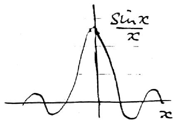
becomes a highly localized, delta-function-like quantity.
That enables the rest of the integrand to be evaluated
just where ∆ω = 0 (i.e. k v0 − ω = 0).
Figure 5.19: Localized integrand function.
So:
|
P = − |
q2 E2
2 m k
|
|
ω
k
|
|
∂f
∂v
| ⎢
⎢
|
[(ω)/k]
|
| ⌠
⌡
|
|
sinx
x
|
d x |
| (5.253) |
Here, x = ∆ωt = ( k v0 − ω) t; but
∫[ sinx/x] d z = π so
|
P = − E2 |
πq2 ω
2 m k2
|
|
∂f0
∂v
| ⎢
⎢
|
[(ω)/k]
|
|
| (5.254) |
We have shown that there is a net transfer of energy to particles
at the resonant velocity [(ω)/k] from the wave.
(Positive if [(∂f)/(∂v)]| is negative.)
5.9.6 Physical Picture
∆ω is minus the wave frequency in the particles' (unperturbed)
frame of reference, or equivalently it is k v0′ where
v0′ is particle speed in wave frame of reference. The
latter is easier to deal with. ∆ωt = k v0′t is the phase the particle travels in time t.
We found that the energy gain was of the form
Figure 5.20: Phase distance traveled in time t.
This integrand becomes small (and oscillatory) for
∆ωt >> 1. Physically, this means that if
particle moves through many wavelengths its energy gain is
small. Dominant contribution is from ∆ωt < π.
These are particles that move through less than 1/2
wavelength during the period under consideration. These are
the resonant particles.
Figure 5.21: Dominant contribution
Particles moving slightly faster than wave are
slowed down. This is a second-order effect.
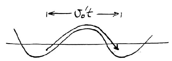
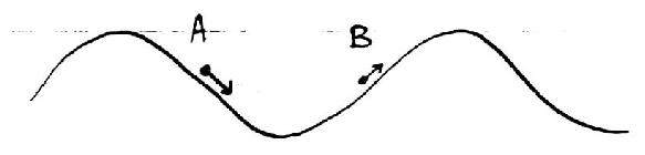
Figure 5.22: Particles moving slightly faster than the wave.
Some particles of the same initial velocity v0 group are being
accelerated (A) some slowed (B). A short time after the wave is
switched on, particles starting at (A) will be moving slightly faster
than those starting at (B). The (A) particles therefore reach the
bottom of the well and stop being accelerated sooner than the (B)
particles reach the top. So (B) particles lose more momentum than (A)
particles gain: on average, faster-than-wave particles are slowed.
Similarly particles moving slightly slower than wave (i.e. from
right to left in the wave frame) are on average speeded up. Net
effect: on average particles move their speed toward that of wave.
But this only continues while particles remain within their initial
potential well: that is, while they have "caught the wave". When
particles have moved half a wavelength their roles are reversed, and
the momentum changes are eventually completely undone after they have
moved a full period.
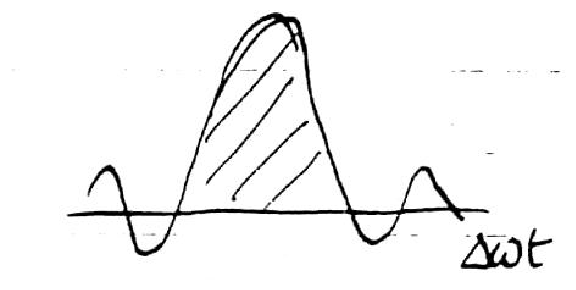
Summary: Resonant particles' velocity is drawn toward
the wave phase velocity.
Is there net energy when we average both slower and faster
particles? Depends which type has most.
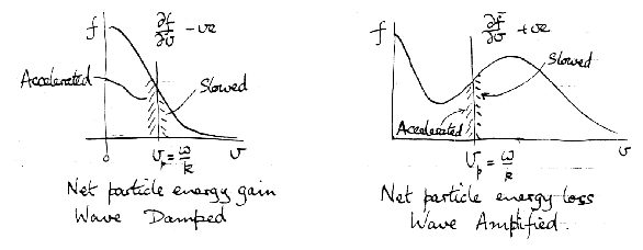
Figure 5.23: Damping or growth depends on distribution slope
Our Complex variables wave treatment and our direct particle
energy calculation give consistent answers. To show this
we need to show energy conservation. Energy density of wave:
|
|
W
|
= |
< sin2 >
|
[ |
Electrostatic
|
+ |
Particle Kinetic
|
] |
| (5.256) |
Magnetic wave energy zero (negligible) for a longitudinal wave.
We showed in Cold Plasma treatment that the velocity due to the wave
is
~v = [q E/(− i ωm )]
Hence
|
|
W
|
≅ |
1
2
|
|
ϵ0 E2
2
|
| ⎡
⎣
|
1 + |
ωp2
ω2
| ⎤
⎦
|
(again electrons only) |
| (5.257) |
When the wave is damped, it has imaginary part of ω,
ωi and
|
|
d t
|
= |
W
|
|
1
E2
|
|
d E2
d t
|
= 2 ωi |
W
|
|
| (5.258) |
Conservation of energy requires that this equal minus
the particle energy gain rate, P. Hence
|
ωi = |
− P
2 W
|
= |
|
+ E2 |
πq2 ω
2 m k2
|
|
∂f0
∂v
| ⎢
⎢
|
[(ω)/k]
|
|
= ωp2 |
π
2
|
|
ω
k2
|
|
1
n
|
|
∂f0
∂v
| ⎢
⎢
|
[(ω)/k]
|
× |
2
|
|
| (5.259) |
So for waves such that ω ∼ ωp, which is the
dispersion relation to lowest order, we get
|
ωi = ωp2 |
π
2
|
|
ωr
k2
|
|
1
n
|
|
∂f0
∂v
| ⎢
⎢
|
[(ωr)/k]
|
. |
| (5.260) |
This exactly agrees with the damping calculated from the complex
dispersion relation using the Vlasov equation.
This is the Landau damping calculation for longitudinal waves in
a (magnetic) field-free plasma. Strictly, just for electron
plasma waves.
How does this apply to the general magnetized plasma case with
multiple species?
Doing a complete evaluation of the dielectric tensor using
kinetic theory is feasible but very heavy algebra. Our direct
intuitive calculation gives the correct answer more directly.
5.9.7 Damping Mechanisms
Cold plasma dielectric tensor is Hermitian. [Complex
conjugate*, transposeT = original matrix.]
This means no damping (dissipation).
The proof of this fact is simple but instructive.
Rate of doing work on plasma per unit volume is P = E. j.
However we need to observe notation.
Notation is that E(k, ω) is amplitude of wave
which is really ℜ(E(k, ω) expi (k . x−ωt)) and similarly for j. Whenever products
are taken: must take real part first. So
| |
|
|
ℜ( Eexpi ( k . x− ωt )) . ℜ( jexpi ( k . x− ωt ) ) |
| |
| |
|
|
|
1
2
|
[ Eeiϕ + E* e−iϕ ] . |
1
2
|
[ jeiϕ + j* e−iϕ ] ( ϕ = k . x− ωt. ) |
| |
| |
|
|
1
4
|
[ E. je2iϕ + E. j* + E* . j+ E* . j* e−2iϕ ] |
| | (5.261) |
|
The terms e2iϕ & e−2iϕ are rapidly
varying. We usually average over at least a period. These
average to zero. Hence
|
< P > = |
1
4
|
[ E. j* + E* . j] = |
1
2
|
ℜ( E. j* ) |
| (5.262) |
Now recognize that j
=σ . E and
substitute
|
< P > = |
1
4
|
[ E.σ* . E* + E* .σ . E] |
| (5.263) |
But for arbitrary matrices and vectors:
(in our dyadic notation we don't explicitly indicate transposes of
vectors). So
hence
|
< P > = |
1
4
|
E* . [ σ*T +σ ] . E |
| (5.266) |
If ϵ = 1 + [ 1/(− i ωϵ0)]σ is
hermitian ϵ*T = ϵ, then the
conductivity tensor is antihermitian σ*T = −σ (if ω is real). In that case,
equation 5.266 shows that 〈P〉 = 0. No dissipation.
Any dissipation of wave energy is associated with a hermitian
part of σ and hence an antihermitian part of
ϵ. Cold Plasma has none.
Collisions introduce damping.
Can be included in equation of motion
|
m |
d v
d t
|
= q ( E+ v∧B) − m v ν |
| (5.267) |
where ν is the collision frequency.
Whole calculation can be followed through replacing
m(−iω) with m(ν− i ω) everywhere.
This introduces complex quantity in S, D, P.
We shall not bother with this because in fusion plasmas
collisional damping is usually negligible. See this
physically by saying that transit time of a wave is
|
|
Size
Speed
|
∼ |
1 meter
3 ×10+8 m/s
|
≅ 3 ×10⁻⁹ seconds. |
| (5.268) |
(Collision frequency)−1 ∼ 10 μs → 1 ms,
depending on Te, ne.
When is the conductivity tensor Antihermitian?
Cold Plasma:
|
ϵ = | ⎡
⎢
⎢
⎢
⎣
|
|
| ⎤
⎥
⎥
⎥
⎦
|
where |
|
S = 1 − |
∑
j
|
|
ωpj2
ω2 − Ωj2
|
|
|
|
D = |
∑
j
|
|
Ωj
ω
|
|
ωpj
ω2 − Ωj2
|
|
|
|
|
|
| (5.269) |
This is manifestly Hermitian if ω is real,
and then σ is anti-Hermitian.
This observation is sufficient to show that if the plasma
is driven with a steady wave, there is no damping, and
k does not acquire a complex part.
Two stream Instability
|
ϵzz = 1 − |
∑
j
|
|
ωpj2
(ω− kvj )2
|
|
| (5.270) |
In this case, the relevant component is Hermitian (i.e. real)
if both ω and k are real.
But that just begs the question: If ω and k are real, then
there's no damping by definition.
So we can't necessarily detect damping or growth just by
inspecting the dieletric tensor form when it depends on
both ω and k.
Electrostatic Waves in general have ϵ = 0 which
is Hermitian. So really it is not enough to deal with
ϵ or χ. We need to deal with σ = − iωϵ0χ, which indeed has a Hermitian component
for the two-stream instability (even though χ is Hermitian)
because ω is complex.
5.9.8 Ion Acoustic Waves and Landau Damping
We previously derived ion acoustic waves based on fluid
treatment giving
Leading to
ω2 ≅ k2 [ [(γiTi + γeTe)/(mi )] ].
Kinetic treatment adds the extra ingredient of Landau Damping.
Vlasov plasma, unmagnetized:
|
ϵzz = 1 − |
ωpe2
k2
|
| ⌠
⌡
|
C
|
|
1
|
|
∂foe
∂v
|
|
dv
n
|
− |
ωpi2
k2
|
| ⌠
⌡
|
C
|
|
1
|
|
∂foi
∂v
|
|
dv
n
|
|
| (5.272) |
Both electron and ion damping need to be considered as
possibly important.
Based on our fluid treatment we know these waves will have
small phase velocity relative to electron
thermal speed. Also cs is somewhat larger than the ion
thermal speed.
Figure 5.24: Distribution functions of ions and
electrons near the sound wave speed.
So we adopt approximations
|
vte >> |
ω
k
|
, vti < ( < ) |
ω
k
|
|
| (5.273) |
and expand in opposite ways.
Ions are in the standard limit, so
|
χi ≅ − |
ωpi2
ω2
|
| ⎡
⎣
|
1 + |
3Ti
m
|
|
k2
ω2
|
+ πi |
ω2
k2
|
|
1
ni
|
|
∂foi
∂v
| ⎢
⎢
|
ω/k
| ⎤
⎦
|
|
| (5.274) |
Electrons: we regard [(ω)/k] as small and write
| |
|
| |
| |
|
|
|
2
n
|
| ⌠
⌡
|
∞
0
|
|
1
v
|
|
∂foe
∂v
|
dv by symmetry |
| |
| |
|
|
|
2
n
|
| ⌠
⌡
|
∞
0
|
− |
me
Te
|
foe dv forMaxwellian. |
| |
| |
|
| | (5.275) |
|
Write F0 = f0 / n.
Contribution from the pole is as usual so
|
χe = − |
ωpe2
k2
|
| ⎡
⎣
|
− |
me
Te
|
+ πi |
∂Foe
∂v
| ⎢
⎢
|
ω/k
| ⎤
⎦
|
|
| (5.276) |
Collecting real and imaginary parts (at real ω)
| |
|
|
1 + |
ωpe2
k2
|
|
me
Te
|
− |
ωpi2
ωr2
|
| ⎡
⎣
|
1 + |
3Ti
m
|
|
k2
ωr2
| ⎤
⎦
|
|
| | (5.277) |
| |
|
| − π |
1
k2
|
| ⎡
⎣
|
ωpe2 |
∂Foe
∂v
| ⎢
⎢
|
ω/k
|
+ ωpi2 |
∂Foi
∂v
| ⎢
⎢
|
ω/k
| ⎤
⎦
|
|
| | (5.278) |
|
The real part is essentially the same as before. The extra
Bohm Gross term in ions appeared previously in the denominator
as
|
|
ωpi2
|
↔ |
ωpi2
ω2
|
| ⎡
⎣
|
1 + |
3Ti
mi
|
|
k2
ω2
| ⎤
⎦
|
|
| (5.279) |
Since our kinetic form is based on a rather inaccurate Taylor
expansion, it is not clear that it is a better approx. We are
probably better off using
Then the solution of ϵr(ωr) = 0 (after some algebra
and using λDe2=(Te/me)/ωpe2) is
|
|
ωr2
k2
|
= | ⎡
⎣
|
3 Ti
mi
|
+ |
1
(1 + k2 λDe2)
|
|
Te
mi
| ⎤
⎦
|
|
| (5.281) |
as before, but we've proved that the correct choice,
keeping the k2λDe2 term
(1st term of ϵr) is γe = 1/(1+k2λDe) ≅ 1.
The imaginary part of ϵ gives damping.
General way to solve for damping when small
We want to solve ϵ(k,ω) = 0 with
ω = ωr + iωi , ωi small.
Taylor expand ϵ about real ωr:
Let ωr be the solution of ϵr(ωr) = 0; then
|
ϵi (ω) = i ϵi (ωr) + i ωi |
∂
∂ωr
|
ϵ(ωr). |
| (5.284) |
This is equal to zero when
If, by presumption, ϵi << ϵr, or more
precisely (in the vicinity of ϵ = 0), ∂ϵi/∂ωr << ∂ϵr/∂ωr then this can
be written to lowest order:
Apply to ion acoustic waves:
|
|
∂ϵr ( ωr )
∂ωr
|
= |
ωpi2
ωr3
|
| ⎡
⎣
|
2 + 4 |
3Ti
mi
|
|
k2
ωr2
| ⎤
⎦
|
|
| (5.287) |
so
|
ωi = |
π
k2
|
|
ωr3
ωpi2
|
| ⎡
⎢
⎣
|
1
| ⎤
⎥
⎦
|
| ⎡
⎣
|
ωpe2 |
∂Foe
∂v
| ⎢
⎢
|
ω/k
|
+ ωpi2 |
∂Foi
∂v
| ⎢
⎢
|
ω/k
| ⎤
⎦
|
|
| (5.288) |
For Maxwellian distributions, using our previous value for ωr,
| |
|
|
| ⎡
⎣
|
− | ⎛
⎝
|
me
2 πTe
| ⎞
⎠
|
1/2
|
|
mev
Te
|
e−[(mev2)/(2Te)] | ⎤
⎦
|
v = [( ωr)/k]
|
|
| |
| |
|
|
|
1
|
| ⎛
⎝
|
me
Te
| ⎞
⎠
|
3/2
|
| ⎡
⎣
|
Te
mi(1+k2λDe2)
|
+ |
3Ti
mi
| ⎤
⎦
|
1/2
|
exp | ⎛
⎝
|
− |
me
2Ti
|
| ⎡
⎣
|
Te
mi(1+k2λDe2)
|
+ |
3Ti
mi
| ⎤
⎦
| ⎞
⎠
|
|
| |
| |
|
|
1
|
| ⎛
⎝
|
me
Te
| ⎞
⎠
|
3/2
|
| ⎡
⎣
|
Te
mi(1+k2λDe2)
|
+ |
3Ti
mi
| ⎤
⎦
|
1/2
|
, |
| | (5.289) |
|
where the exponent is of order me/mi here,
and so the exponential is ≅ 1. And for ions
|
|
∂Foi
∂v
| ⎢
⎢
|
[(ωr)/k]
|
= − |
1
|
|
mi
Ti
|
| ⎡
⎣
|
1
1 + k2 λD2
|
+ |
3Ti
Te
| ⎤
⎦
|
1/2
|
| ⎛
⎝
|
Te
Ti
| ⎞
⎠
|
1/2
|
exp | ⎛
⎝
|
− | ⎡
⎣
|
Te
2Ti
|
|
1
1 + k2 λD2
|
+ |
3
2
| ⎤
⎦
| ⎞
⎠
|
|
| (5.290) |
Hence
| |
|
|
|
π
|
|
ωr2
k2
|
| ⎡
⎢
⎣
|
1
| ⎤
⎥
⎦
|
| ⎡
⎣
|
1
1 + k2 λD2
|
+ |
3Ti
Te
| ⎤
⎦
|
1/2
|
× |
| |
| |
|
|
| ⎡
⎣
|
mi
me
|
| ⎛
⎝
|
me
mi
| ⎞
⎠
|
1/2
|
|
me
Te
|
+ |
mi
Ti
|
| ⎛
⎝
|
Te
Ti
| ⎞
⎠
|
1/2
|
exp | ⎛
⎝
|
− |
Te
2Ti
|
|
1
1 + k2 λD2
|
− |
3
2
| ⎞
⎠
| ⎤
⎦
|
|
| |
| |
|
|
|
⎛
√
|
|
| ⎡
⎢
⎣
|
1
| ⎤
⎥
⎦
|
| ⎡
⎣
|
1
1 + k2 λD2
|
+ |
3Ti
Te
| ⎤
⎦
|
3/2
|
× |
| |
| |
|
| ⎡
⎣
|
|
electron
|
+ |
|
| ⎛
⎝
|
Te
Ti
| ⎞
⎠
|
3/2
|
exp | ⎛
⎝
|
− |
Te
2Ti
|
|
1
1 + k2 λD2
|
− |
3
2
| ⎞
⎠
|
|
ion Landau damping
|
| ⎤
⎦
|
. |
| | (5.291) |
|
[Note: the coefficient on the first line of equation 5.291 for
ωi/ωr
reduces to ≅ −√{π/8} for Ti/Te << 1 and kλDe << 1.]
Electron Landau damping of ion acoustic waves is rather small:
[(ωi)/(ωr)] ∼ √{[(me)/(mi)]} ∼ [1/70].
Ion Landau damping is large, ∼ 1 unless the term in
the exponent is large. That is
Physics is that large [(Te)/(Ti)] pulls the phase
velocity of the wave:
√{ [(Te + 3Ti)/(mi )]} = cs
above the ion thermal velocity
vti = √{[(Ti)/(mi)]}.
If cs >> vti there are few resonant ions to damp
the wave.
[Note. Many texts drop terms of order
[(Ti)/(Te)] early in the treatment,
but that is not really accurate. We have kept
the [(Ti)/(Te)] to first order, giving an extra leading coefficient
|
| ⎡
⎢
⎣
|
2
| ⎤
⎥
⎦
|
| ⎡
⎣
|
1
1 + k2 λD2
|
+ |
3Ti
Te
| ⎤
⎦
|
3/2
|
≅ | ⎡
⎣
|
1 + 3Ti/Te
1 + 6Ti/Te
| ⎤
⎦
|
| ⎡
⎣
|
1 + |
3Ti
Te
| ⎤
⎦
|
3/2
|
≅ 1 + |
3
2
|
|
Ti
Te
|
|
| (5.293) |
and an extra term −3/2 in the
exponent.
When Ti ∼ Te we ought really to use full solutions
based on the Plasma Dispersion Function.]
5.9.9 Alternative expressions of Dielectric Tensor
Elements
This subsection gives some useful algebraic relationships that enable
one to transform to different expressions sometimes encountered.
| |
|
|
|
q2
ωmϵ0
|
| ⌠
⌡
|
C
|
|
ω− kv
|
dv = |
q2
ω2 mϵ0
|
|
ω
k
|
| ⌠
⌡
|
C
|
| ⎛
⎝
|
ω
ω− kv
|
− 1 | ⎞
⎠
|
|
∂f0
∂v
|
dv |
| | (5.294) |
| |
|
|
|
q2
mϵ0
|
|
1
k2
|
| ⌠
⌡
|
C
|
|
1
|
|
∂f0
∂v
|
dv |
| | (5.295) |
| |
|
|
|
ωp2
k2
|
| ⌠
⌡
|
C
|
|
1
|
|
1
n
|
|
∂f0
∂v
|
dv |
| | (5.296) |
| |
|
|
ωp2
k2
|
| ⎡
⎢
⎣
|
℘ | ⌠
⌡
|
|
1
|
|
∂F0
∂v
|
dv − πi |
∂F0
∂v
| ⎢
⎢
|
[(ω)/k]
| ⎤
⎥
⎦
|
|
| | (5.297) |
|
where F0 = [(f0)/n] is the normalized distribution
function. Other elements of χ involve
integrals of the form
|
χjl |
ωm ϵ0
q2
|
= | ⌠
⌡
|
|
ω− k . v
|
d3 v . |
| (5.298) |
When k is in z-direction, k.v = kzvz.
(Multi dimensional distribution f0).
If (e.g., χxy) l ≠ z and
j ≠ l then the integral over vl yields
∫[(∂f0)/(∂vl)] dvl = 0.
If j = l ≠ z then
|
| ⌠
⌡
|
vj |
∂f0
∂vj
|
dvj = − | ⌠
⌡
|
f0dvj , |
| (5.299) |
by parts. So, recalling the definition fz ≡ ∫f dvx dvy,
| |
|
|
− |
q2
ωm ϵ0
|
| ⌠
⌡
|
|
foz
ω− k.v
|
dvz |
| |
| |
|
| − |
ωp2
ω
|
| ⌠
⌡
|
|
Foz
ω− k . v
|
dvz. |
| | (5.300) |
|
The fourth type of element is
|
χxz = |
q2
ωm ϵ0
|
| ⌠
⌡
|
|
ω− kzvz
|
d3 v . |
| (5.301) |
This is not zero unless f0 is isotropic ( = f0(v)).
If f is isotropic
|
|
∂f0
∂vz
|
= |
d f0
d v
|
|
∂v
∂vz
|
= |
vz
v
|
|
d f0
d v
|
|
| (5.302) |
Then
| |
|
|
| ⌠
⌡
|
|
vx vz
ω− kz vz
|
|
1
v
|
|
d f0
dv
|
d3 v |
| |
| |
|
| ⌠
⌡
|
|
vz
ω− kz vz
|
|
∂f0
∂vx
|
d3 v = 0 |
| | (5.303) |
|
(since the vx-integral of ∂f0/∂vx is zero). Hence
for isotropic F0=f0/n, with k in the z-direction,
|
χ = | ⎡
⎢
⎢
⎢
⎢
⎢
⎢
⎢
⎣
|
|
− |
ωp2
ω
|
| ⌠
⌡
|
C
|
|
Foz
ω− k vz
|
dvz |
| | |
| |
− |
ωp2
ω
|
| ⌠
⌡
|
C
|
|
Foz
ω− k vz
|
dvz |
| |
| | |
|
ωp2
k
|
| ⌠
⌡
|
C
|
|
1
ω− k vz
|
|
∂Foz
∂vz
|
dvz |
|
|
| ⎤
⎥
⎥
⎥
⎥
⎥
⎥
⎥
⎦
|
|
| (5.304) |
(and the terms 0+ are the ones that need isotropy to
make them zero).
where
| |
|
|
1 − |
ωp2
ω
|
| ⌠
⌡
|
C
|
|
Foz
ω− kvz
|
dvz |
| | (5.306) |
| |
|
| 1 − |
ωp2
k2
|
| ⌠
⌡
|
C
|
|
1
|
|
∂Foz
∂vz
|
dvz |
| | (5.307) |
|
All integrals are along the
Landau contour, passing below the pole.
5.9.10 Electromagnetic Waves in unmagnetized Vlasov Plasma
For transverse waves the dispersion relation is
|
|
k2c2
ω2
|
= N2 = ϵt = 1 − |
ωp2
ω
|
|
1
n
|
| ⌠
⌡
|
C
|
|
foz dvz
( ω− kzvz )
|
|
| (5.308) |
This has, in principle, a contribution from the pole at
ω− kvz = 0. However, for a non-relativistic
plasma, thermal velocity is << c and the EM wave has
phase velocity ∼ c. Consequently, for all velocities
vz for which foz is non-zero kvz << ω.
We have seen with the cold
plasma treatment that the wave phase velocity is actually greater than c.
Therefore a proper relativistic distribution function will have
no particles at all in resonance with the wave.
Therefore:
- The imaginary part of ϵt from the pole
is negligible. And relativistically zero.
-
| |
|
|
1 − |
ωp2
ω2
|
|
1
n
|
| ⌠
⌡
|
∞
−∞
|
foz | ⎛
⎝
|
1 + |
kvz
ω
|
+ |
k2 vz2
ω2
|
+... | ⎞
⎠
|
dvz |
| |
| |
|
|
1 − |
ωp2
ω2
|
| ⎡
⎣
|
1 + |
k2
ω2
|
|
T
m
|
+ ... | ⎤
⎦
|
|
| |
| |
|
|
1 − |
ωp2
ω2
|
| ⎡
⎣
|
1 + |
k2 vt2
ω2
| ⎤
⎦
|
|
| |
| |
|
| | (5.309) |
|
Thermal correction to the refractive index N is small because
[(k2vt2)/(ω2)] << 1.
Electromagnetic waves are hardly affected by Kinetic Theory
treatment in unmagnetized plasma. Cold Plasma treatment is
generally good enough.
5.10 Experimental Verification of Landau Damping
This last section consists of viewgraphs that may be viewed
at expts.pdf.