Chapter 4
Fluid Description of Plasma
The single particle approach gets to be horribly complicated, as we
have seen.
Basically we need a more statistical approach because we can't
follow each particle separately. If the details of the distribution
function in velocity space are important we have to stay with the
Boltzmann equation. It is a kind of particle conservation equation.
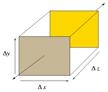
4.1 Particle Conservation (In 3-d Space)
Figure 4.1: Elementary volume for particle conservation
Number of particles in box ∆x ∆y ∆z is the volume,
∆V = ∆x ∆y ∆z, times the density n. Rate
of change of number is is equal to the number flowing across the
boundary per unit time, the flux. (In absence of sources.)
|
− |
∂
∂t
|
[∆x ∆y ∆z n] = Flow Out across boundary. |
| (4.1) |
Take particle velocity to be v(r) [no random velocity,
only flow] and origin at the center of the box refer to flux density
as nv
= Γ.
|
Flow Out = [Γz ( 0, 0, ∆z/2 ) − Γz ( 0, 0, −∆z/2 ) ] ∆x ∆y + x + y . |
| (4.2) |
Expand as Taylor series
|
Γz (0, 0, η) = Γz (0) + |
∂
∂z
|
Γz . η |
| (4.3) |
So,
| |
|
|
|
∂
∂z
|
(n vz) ∆z ∆x∆y + x + y |
| | (4.4) |
| |
|
| |
|
Hence Particle Conservation
Notice we have essential proved an elementary form of Gauss's
theorem
|
| ⌠
⌡
|
v
|
∇ . A d3 r = | ⌠
⌡
|
∂V
|
A . dS . |
| (4.6) |
The expression: `Fluid Description' refers to any
simplified plasma treatment which does not keep track
of v-dependence of f detail.
- Fluid Descriptions are essentially 3-d (r).
- Deal with quantities averaged over velocity space
(e.g. density, mean velocity, ...).
- Omit some important physical processes (but describe
others).
- Provide tractable approaches to many problems.
Fluid Equations can be derived mathematically by taking
moments1 of the Boltzmann Equation.
These lead, respectively, to (0) Particle (1) Momentum (2) Energy
conservation equations.
We shall adopt a more direct `physical' approach.
4.2 Fluid Motion
The motion of a fluid is described by a vector velocity field
v(r) (which is the mean velocity of all the individual
particles which make up the fluid at r). Also the particle
density n(r) is required. We are here discussing the motion of
fluid of a single type of particle of mass/charge,
m/q so the charge and mass density are qn and mn
respectively.
The particle conservation equation we already know. It is also
sometimes called the `Continuity Equation'
It is also possible to expand the ∇. to get:
|
|
∂
∂t
|
n + (v. ∇) n + n ∇ . v= 0 |
| (4.11) |
The significance, here, is that the first two terms are
the `convective derivative" of n
|
|
D
Dt
|
≡ |
d
dt
|
≡ |
∂
∂t
|
+ v. ∇ |
| (4.12) |
so the continuity equation can be written
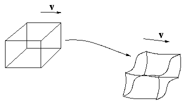
4.2.1 Lagrangian & Eulerian Viewpoints
There are essentially 2 views.
- Lagrangian. Sit on a fluid element and move
with it as fluid moves.
Figure 4.2: Lagrangean Viewpoint
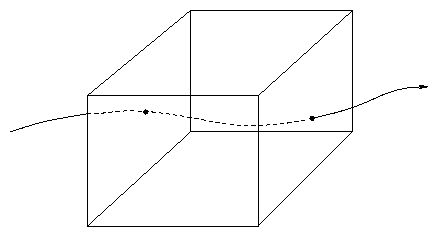
- Eulerian. Sit at a fixed point in space and
watch fluid move through your volume element: "identity" of fluid in volume
continually changing
Figure 4.3: Eulerian Viewpoint
[(∂)/(∂t)] means rate of change at fixed
point (Euler).
[ D/Dt] ≡ [d/dt] ≡ [( ∂)/(∂t )] + v. ∇ means rate of change at
moving point (Lagrange).
v.∇ = [dx/(∂t)] [(∂)/(∂x)]+[dy/(∂t)] [(∂)/(∂y)]+[dz/(∂t)] [(∂)/(∂z)]
: change due to motion of observation point.
Our derivation of continuity was Eulerian. From the Lagrangian
view
|
|
D
Dt
|
n = |
d
dt
|
|
∆N
∆V
|
= − |
∆N
∆V2
|
|
d
dt
|
∆V = − n |
1
∆V
|
|
d ∆V
dt
|
|
| (4.14) |
since total number of particles in volume element (∆N) is
constant (we are moving with them). (∆V = ∆x ∆y ∆z.)
| |
|
|
|
d∆x
dt
|
∆y ∆z + |
d ∆y
dt
|
∆z ∆x + |
d ∆z
dt
|
∆y ∆x |
| | (4.15) |
| |
|
| ∆V | ⎡
⎣
|
1
∆x
|
|
d ∆x
dt
|
+ |
1
∆y
|
|
d ∆y
dt
|
+ |
1
∆x
|
|
d ∆z
dt
| ⎤
⎦
|
|
| | (4.16) |
|
| |
|
|
vx ( ∆x / 2 ) − vx ( − ∆x / 2 ) |
| | (4.17) |
| |
|
| ∆x |
∂vx
∂x
|
etc. ... y ... z |
| | (4.18) |
|
Hence
|
|
d
dt
|
∆V = ∆V | ⎡
⎣
|
∂vx
∂x
|
+ |
∂vy
∂y
|
+ |
∂vz
∂z
| ⎤
⎦
|
= ∆V ∇ . v |
| (4.19) |
and so
Lagrangian Continuity. Naturally, this is the same equation
as Eulerian when one puts
[D/Dt] = [(∂)/(∂t)] + v. ∇.
The quantity − ∇ . v is the rate of (Volume) compression of
element.
4.2.2 Momentum (Conservation) Equation
Each of the particles is acted on by the Lorentz force
q [E+ ui ∧B] (ui is
individual particle's velocity).
Hence total force on the fluid element due to E-M fields is
|
|
∑
i
|
( q [ E+ ui ∧B
] ) = ∆N q ( E+ v∧B) |
| (4.21) |
(Using mean: v
= ∑i ui / ∆N.)
E-M Force density (per unit volume) is:
The total momentum of the element is
|
|
∑
i
|
m ui = m ∆N v
= ∆V mn v
|
| (4.23) |
so Momentum Density is mnv.
If no other forces are acting then clearly the equation of motion
requires us to set the time derivative of mnv equal
to FEM. Because we want to retain the identity
of the particles under consideration we want D/Dt i.e.
the convective derivative (Lagrangian picture).
In general there are additional forces acting.
(1) Pressure (2) Collisional Friction.
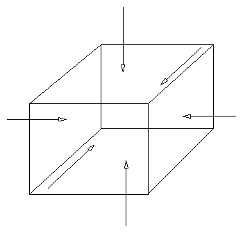
4.2.3 Pressure Force
In a gas p( = nT) is the force per unit area arising from
thermal motions. The surrounding fluid exerts this force on
the element:
Figure 4.4: Pressure forces on opposite faces of element.
Net force in x direction is
| |
|
|
p ( ∆x / 2 ) ∆y ∆z + p ( − ∆x / 2 ) ∆y ∆z |
| | (4.24) |
| |
|
| − ∆x ∆y ∆z |
∂p
∂x
|
= − ∆V |
∂p
∂x
|
= − ∆V ( ∇p )x |
| | (4.25) |
|
So (isotropic) pressure force density (/unit vol)
How does this arise in our picture above?
Answer: Exchange of momentum by particle
thermal motion across the element boundary.
Although in Lagrangian picture we move with the element
(as defined by mean velocity v) individual particles
also have thermal velocity so that the additional
velocity they have is
|
wi = ui − v `peculiar′velocity |
| (4.27) |
Because of this, some cross the element boundary and
exchange momentum with outside. (Even though there is
no net change of number of particles in element.)
Rate of exchange of momentum due to particles with peculiar
velocity w, d3w across a surface element
ds is
|
|
f( w ) m w d3 w
momentum density at w
|
× |
w . ds
flow rate across ds
|
|
| (4.28) |
Integrate over distrib function to obtain the total
momentum exchange rate:
The thing in the integral is a tensor. Write
|
p = | ⌠
⌡
|
m w w f (w) d3w (Pressure Tensor) |
| (4.30) |
Then momentum exchange rate is
Actually, if f(w) is isotropic (e.g. Maxwellian) then
| |
|
|
| ⌠
⌡
|
m wx wy f (w) d3w = 0 etc. |
| | (4.32) |
| |
|
| ⌠
⌡
|
m wx2 f (w) d3w ≡ n T ( = pyy = pzz = `p′) |
| | (4.33) |
|
So then the exchange rate is pds. (Scalar Pressure).
Integrate ds over the whole ∆V then x
component of momm exchange rate is
|
p | ⎛
⎝
|
∆x
2
| ⎞
⎠
|
∆y ∆z− p | ⎛
⎝
|
− ∆x
2
| ⎞
⎠
|
∆y ∆z = ∆V ( ∇ p )x |
| (4.34) |
and so
Total momentum loss rate due to exchange across the boundary
per unit volume is
In terms of the momentum equation, either we put ∇p on the
momentum derivative side or Fp on force side. The result
is the same.
Ignoring Collisions, Momentum Equation is
|
|
D
Dt
|
( m n ∆V v) = [FEM + Fp ] ∆V |
| (4.36) |
Recall that n∆V = ∆N ; [D/Dt] (∆N) = 0; so
|
|
D
Dt
|
( m n ∆V v) = m n ∆V |
Dv
dt
|
. |
| (4.37) |
Thus, substituting for F′s:
Momentum Equation.
|
m n |
Dv
Dt
|
= m n | ⎛
⎝
|
∂v
∂t
|
+ v. ∇ v | ⎞
⎠
|
= q n ( E + v∧B) − ∇p |
| (4.38) |
4.2.4 Momentum Equation: Eulerian Viewpoint
Fixed element in space. Plasma flows through it.
- E.M. force on element (per unit vol.)
|
FEM = nq ( E+ v∧B) as before. |
| (4.39) |
- Momentum flux across boundary (per unit vol)
| |
|
|
∇. | ⌠
⌡
|
m (v+ w) (v+ w) f(w) d3w |
| | (4.40) |
| |
|
|
∇. { | ⌠
⌡
|
m (vv+ |
vw + wv
integrates to 0
|
+ w w) f(w) d3 w } |
| | (4.41) |
| |
|
| | (4.42) |
| |
|
| m n (v. ∇) v+ m v[ ∇ . (n v) ] + ∇p |
| | (4.43) |
|
(Take isotropic p.)
- Rate of change of momentum within element (per unit vol)
Hence, total momentum balance in what is called "conservation form"
|
|
∂
∂t
|
(m n v) + ∇.(mnvv+pI ) = FEM |
| (4.45) |
To render into Lagrangean form, use the continuity equation
to cancel the second term of (4.43) and part of the
∂/∂t term as follows
|
|
∂
∂t
|
(m n v) + m v( ∇ . ( n v) ) = m v{ |
∂n
∂t
|
+ ∇ . ( n v) } + m n |
∂v
∂t
|
= m n |
∂v
∂t
|
|
| (4.47) |
Then take ∇p to RHS to get final form:
Momentum Equation:
|
m n | ⎡
⎣
|
∂v
∂t
|
+ ( v. ∇ ) v | ⎤
⎦
|
= nq ( E+ v∧B) − ∇p . |
| (4.48) |
As before, via Lagrangian formulation. (Collisions
have been ignored.)
4.2.5 Effect of Collisions
First notice that like particle collisions
do not change the total momentum (which is
averaged over all particles of that species).
Collisions between unlike particles do
exchange momentum between the species. Therefore once
we realize that any quasi-neutral plasma consists of
at least two different species (electrons and ions) and
hence two different interpenetrating fluids we may need
to account for another momentum loss (gain) term.
The rate of momentum density loss by species 1 colliding
with species 2 is:
Hence we can immediately generalize the momentum
equation to
|
m1 n1 | ⎡
⎣
|
∂v1
∂t
|
+ ( v1 . ∇ ) v1 | ⎤
⎦
|
= n1 q1 ( E+ v1 ∧B) − ∇p1 − ν12 n1 m1 ( v1 − v2 ) |
| (4.50) |
With similar equation for species 2.
4.3 The Key Question for Momentum Equation:
What do we take for p?
Basically p = nT is determined by energy balance, which
will tell how T varies. We could write an energy equation
in the same way as momentum. However, this would then contain a
term for heat flux, which would be unknown. In general, the
kth moment equation contains a term which is a
(k + 1)th moment.
Continuity, 0th equation contains v determined by
Momentum, 1st equation contains p determined by
Energy, 2nd equation contains Q determined by ...
In order to get a sensible result we have to truncate
this hierarchy. Do this by some sort of assumption about the
heat flux. This will lead to an
Equation of State:
The value of γ to be taken depends on the heat flux assumption
and on the isotropy (or otherwise) of the energy distribution.
Examples
- Isothermal: T = const.: γ = 1.
- Adiabatic/Isotropic: 3 degrees of freedom γ = 5/3.
- Adiabatic/1 degree of freedom γ = 3.
- Adiabatic/2 degrees of freedom γ = 2.
In general, energy conservation is n (l/ 2) δT = − p (δV/V)
(Adiabatic l degrees)
So
| |
|
|
δn
n
|
+ |
δT
T
|
= | ⎛
⎝
|
1 + |
2
l
| ⎞
⎠
|
|
δn
n
|
, |
| | (4.53) |
|
i.e.
|
p n −( 1 + [2/(l)]) = const. |
| (4.54) |
In a normal gas, which `holds together' by collisions, energy is
rapidly shared between 3 space-degrees of freedom. Plasmas are
often rather collisionless so compression in 1 dimension often
stays confined to 1-degree of freedom. Sometimes heat
transport is so rapid that the isothermal approach is valid.
It depends on the exact situation; so let's leave γ undefined
for now.
4.4 Summary of Two-Fluid Equations
Species j
Plasma Response
- Continuity:
- Momentum:
|
mjnj | ⎡
⎣
|
∂vj
∂t
|
+ ( vj . ∇ ) vj | ⎤
⎦
|
= njqj ( E+ vj ∧B) − ∇pj − |
-
ν
|
jk
|
njmj (vj − vk ) |
| (4.56) |
- Energy/Equation of State:
(j = electrons, ions).
Maxwell's Equations
| |
|
| | (4.58) |
| |
|
| μo j + |
1
c2
|
|
∂E
∂t
|
∇ ∧E
= |
−∂B
∂t
|
|
| | (4.59) |
|
With
| |
|
|
qe ne + qi ni = e ( −ne + Zni ) |
| | (4.60) |
| |
|
|
qe ne ve + qi ni vi = e ( −ne ve + Z ni vi ) |
| | (4.61) |
| |
|
| −e ne ( ve − vi r) (Quasineutral) |
| | (4.62) |
|
Accounting
| Unknowns
| Equations |
| ne,ni | 2 | Continuity e, i | 2 |
| ve,vi | 6 | Momentum e,i | 6 |
| pe,pi | 2 | State e,i | 2 |
| E, B | 6 | Maxwell | 8 |
| 16 | | 18 |
but 2 of Maxwell (∇. equs) are redundant
because can be deduced from others:
e.g.
| |
|
| | (4.63) |
| |
|
| 0 = μo ∇ . j + |
1
c2
|
|
∂
∂t
|
( ∇ . E) = |
1
c2
|
|
∂
∂t
|
| ⎛
⎝
|
−ρ
ϵo
|
+ ∇ . E | ⎞
⎠
|
|
| | (4.64) |
|
So 16 equs for 16 unknowns.
Equations still very difficult and complicated mostly because
it is Nonlinear
In some cases can get a tractable problem by `linearizing'.
That means, take some known equilibrium solution and suppose
the deviation (perturbation) from it is small so we can retain
only the 1st linear terms and not the others.
4.5 Two-Fluid Equilibrium: Diamagnetic Current
Slab: [(∂)/(∂x)] ≠ 0 [(∂)/(∂y)], [(∂)/(∂z)] = 0.
Straight B-field: B
= B∧z.
Equilibrium: [(∂)/(∂t)] = 0 (E = − ∇ϕ)
Collisionless: ν→ 0.
Momentum Equation(s):
|
mjnj (vj . ∇) vj = nj qj (E+ vj ∧B) − ∇pj |
| (4.65) |
Drop j suffix for now. Then take x,y components:
Eq 4.67 is satisfied by taking vx = 0.
Then 4.66 →
|
nq (Ex + vy B) − |
dp
dx
|
= 0. |
| (4.68) |
i.e.
|
vy = |
− Ex
B
|
+ |
1
nqB
|
|
dp
dx
|
|
| (4.69) |
or, in vector form:
|
v= |
E∧B drift
|
− |
Diamagnetic Drift
|
|
| (4.70) |
Notice:
- In magnetic field (⊥) fluid velocity is determined
by component of momentum equation orthogonal to it
(and to B).
- Additional drift (diamagnetic) arises in standard
F ∧B form from pressure force.
- Diagmagnetic drift is opposite for opposite signs of
charge (electrons vs. ions).
Now restore species distinctions and consider electrons
plus single ion species i. Quasineutrality says
niqi = −neqe.
Hence adding solutions
|
neqeve + niqivi = |
E∧B
B2
|
|
( niqi + neqe )
=0
|
− ∇( pe + pi )∧ |
B
B2
|
|
| (4.71) |
Hence current density:
|
j = − ∇( pe + pi ) ∧ |
B
B2
|
|
| (4.72) |
This is the diamagnetic current. The electric field, E, disappears
because of quasineutrality.
(General case ∑j qjnjvj = − ∇(∑pj) ∧B/ B2).
4.6 Two-Fluid Dynamics
We shall see that two-fluid treatments are widely used the question of
waves, but before we get into that in detail, let us look briefly at
some time-varying situations for two-fluid treatments.
4.6.1 Parallel Two-Fluid Dynamics
When motion is in the parallel-to-B direction, the fluid momentum
equation becomes
|
m n | ⎡
⎣
|
∂
∂t
|
+ v |
∂
∂ z
| ⎤
⎦
|
v = nq E − |
∂p
∂z
|
, |
| (4.73) |
where z is the parallel coordinate, all components are parallel, and
perpendicular variation is taken to be absent.
An equation like this applies to both the electrons and ions. Now
consider a one-dimensional compression of the plasma so that the
density varies with z. Start with electrons. They are very light
compared with ions, so if the time derivative is relatively slow, the
rate of change of their momentum, which is the left hand side of this
equation, is negligible. Also, since their rapid thermal conduction
along the field lines will oppose any temperature variation let us
suppose that the electron temperature Te is uniform. (That's our
equation of state for electrons). In that case
as an approximation we can write
|
−qe |
∂ϕ
∂z
|
=qe E = |
1
ne
|
|
∂ p
∂z
|
= |
Te
ne
|
|
∂ ne
∂z
|
= Te |
∂ln(ne)
∂z
|
. |
| (4.74) |
This equation can simply be integrated from some arbitrary reference
point where ϕ = 0 and ne=ne0 to find ln(ne/ne0) = −qeϕ/Te or
This is the Boltzmann factor that we invoked for a thermal equilibrium
situation at the beginning of the course. We see that the fluid
equations derive the same variation along the magnetic field, assuming
the electrons to be in equilibrium. The pressure gradient term and the
electric force balance each other.
Now what about the ions? We cannot ignore their inertia because they
are heavy. But let us suppose that they have only a very small
velocity so that the second-order convective derivative term can be
ignored, and only mini∂vi/∂t remains on the left hand side
of eq. (4.73). Using our solution for the
relationship between ϕ and ne, which implies ∂ϕ/∂z = (e/ne)∂ne/∂z we can then write the ion
momentum equation as
|
mini |
∂vi
∂t
|
=niqiE − |
∂ pi
∂z
|
= |
niqi
neqe
|
Te |
∂ne
∂ z
|
− |
∂pi
∂z
|
|
| (4.76) |
We now recognize the effect of quasi-neutrality is that there can
be very little difference between −qene and qini, so we set
them equal (this is sometimes called the "plasma
approximation"). Also, if the ion equation of state is
pi ni−γi = constant, then we can write
|
|
∂pi
∂z
|
= γi |
pi
ni
|
|
∂ ni
∂z
|
= γiTi |
∂ni
∂z
|
|
| (4.77) |
and the momentum equation becomes
|
ρi |
∂vi
∂t
|
= −(Z Te+γiTi) |
∂ ni
∂z
|
, |
| (4.78) |
where Z=|qi/qe| is the ion charge-number and ρi=nimi is
the ion mass density.
This ion momentum equation is of just the form that a standard gas
would have, except that instead of just γT we have
ZTe+γi Ti. It states
that the ion fluid has a rate of change of momentum density equal to
minus a pressure gradient. But the pressure gradient involves not just
the ion pressure, it also involves the electron pressure. What is
happening is that the electron pressure gradient is being sustained by
the ion inertia because the electric field (through ϕ) transfers
force between the electrons and the ions.
To complete the physics we need the continuity equation
|
|
∂ni
∂t
|
= − |
∂(ni vi)
∂ z
|
≅ − ni |
∂vi
∂ z
|
, |
| (4.79) |
(ignoring vi∂ni/∂z as second order assuming small
variation of ni and small vi) which allows us to derive a
combined partial differential equation for each perturbed quantity
alone, for example eliminate vi and we get an equation for ni:
|
|
∂2 ni
∂t2
|
≅ | ⎡
⎣
|
ZTe+γi Ti
mi
| ⎤
⎦
|
|
∂2 ni
∂z2
|
≡ cs2 |
∂2 ni
∂z2
|
. |
| (4.80) |
This can easily be recognized as a one dimensional wave equation
whose speed of propagation (cs) squared is the square bracket. This is
called the ion sound (or acoustic) speed.
Warning This fluid treatment turns out to omit an
important part (ion Landau damping) of the physics of longitudinal
acoustic oscillations , as we will see later when we do a kinetic
theory treatment. The fluid treatment is valid only when Ti << Te,
in which case the sound speed is cs=√{ZTe/mi}, and only the
electron pressure matters.
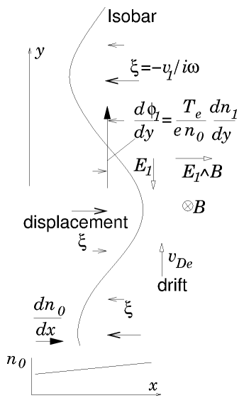
4.6.2 Drift Waves
Figure 4.5: Mechanism of driftwaves
A another type of wave that requires two-fluids for its existence
depends upon a density gradient. Consider a configuration like that
used to discuss the diamagnetic drifts, where there is a background
density (n0) gradient only in the x-direction
[(∂n)/(∂x)]=n0′ (temperatures are taken uniform
for simplicity). Suppose there is a perturbative velocity v1 in the
x-direction that is independent of x but varies sinusoidally in
the y-direction and in time so v1 ∝ expi(ky−ωt) and
similar small perturbations arise in the other parameters too: n1
and ϕ1. We will suppose that the magnetic field is almost
entirely in the z-direction, except that there is a tiny but
sufficient By component to allow us to use the electron parallel
pressure balance equation to conclude that the electron density is
governed by the Boltzmann factor n ∝ exp(eϕ/Te), but not
enough By to affect anything else. For small perturbative
displacements (dropping second order terms like n1v1) the
continuity equation is
|
|
∂n1
∂t
|
= −iωn1=− |
∂
∂ x
|
(nv) ≅ −v1 n0′. |
| (4.81) |
The Boltzmann factor relates the value of n1 to ϕ1 from
eϕ1/Te = n1/n0. But why would there be any v1 in the
x-direction? Because there is a potential gradient in the y
direction giving Ey=−[(∂ϕ1)/(∂y)]=−ikϕ1,
and consequently an E∧B drift (noting Bz=−B)
We therefore have a self-consistent solution when
|
ik |
ϕ1
B
|
=v1 = iω |
n1
n0′
|
= iω |
eϕ1
Te
|
|
n0
n0′
|
. |
| (4.83) |
Cancelling ϕ1 from the first and last expression
we find the "dispersion relation", which relates
ω and k:
|
|
ω
k
|
= |
Te
eB n0
|
|
∂n0
∂x
|
=vDe. |
| (4.84) |
This expression shows the phase velocity ω/k is exactly the
diamagnetic drift velocity of the electrons (see eq. 4.70). So we have found that
there exist waves consisting of transverse displacement (velocity)
perpendicular to B and k that propagate at the velocity of the
electron diamagnetic drift. Notice that these waves have v1 exactly
90 degrees out of phase (multiplied by i) with respect to ϕ1
and n1. If some other physics (for example finite parallel
resistivity) intervenes in addition giving rise to a change of this
phase shift, these waves can become unstable.
4.7 Reduction of Fluid Approach to the Single Fluid
Equations
So far we have been using fluid equations which apply to
electrons and ions separately. These are called
`Two Fluid' equations because we always have to keep
track of both fluids separately.
A further simplification is possible and useful sometimes
by combining the electron and ion equations together to
obtain equations governing the plasma viewed as a
`Single Fluid'.
Recall 2-fluid equations:
| |
|
| | (4.85) |
| |
|
| mjnj | ⎛
⎝
|
∂
∂t
|
+ vj . ∇ | ⎞
⎠
|
vj = njqj ( E+ vj ∧B) − ∇pj + Fjk |
| | (4.86) |
|
(where we just write Fjk = −―vjknjmj ( vj − vk ) for short.)
Now we rearrange these 4 equations (2 × 2 species) by
adding and subtracting appropriately to get new equations
governing the new variables:
| |
|
| | (4.87) |
| |
|
|
( neme ve + nimivi ) / ρm |
| | (4.88) |
| |
|
| | (4.89) |
| |
Electric Current Density j |
|
|
| | (4.90) |
| |
|
|
qe ne ( ve−vi ) by quasi neutrality |
| | (4.91) |
| |
|
| | (4.92) |
|
1st equation: take me ×Ce + mi ×Ci →
|
(1) |
∂ρm
∂t
|
+ ∇ . ( ρm V ) = 0 Mass Conservation |
| (4.93) |
2nd take qe ×Ce + qI ×Ci →
|
(2) |
∂ρq
∂t
|
+ ∇ . j = 0 Charge Conservation |
| (4.94) |
3rd take Me + Mi. This is a bit more difficult.
RHS becomes:
|
|
∑
| njqj ( E+ vj ∧B) − ∇pj + Fjk = ρq E+ j ∧B− ∇( pe + pi ) |
| (4.95) |
(we use the fact that
Fei − Fie so no net friction).
LHS is
|
|
∑
j
|
mj nj | ⎛
⎝
|
∂
∂t
|
+ vj .∇ | ⎞
⎠
|
vj . |
| (4.96) |
The difficulty here is that the convective term is non-linear and so
does not easily lend itself to reexpression in terms of the new
variables. But note that since me << mi the contribution from
electron momentum is much less than that from ions and we can usually
ignore it in this equation. Also to the same degree of approximation
(dropping terms of order me/mi) V ≅ vi: the
CM velocity is the ion velocity. Thus for the LHS of this momentum
equation we take
|
|
∑
j
|
mini | ⎛
⎝
|
∂
∂t
|
+ vj . ∇ | ⎞
⎠
|
vj ≅ ρm | ⎛
⎝
|
∂
∂t
|
+ V . ∇ | ⎞
⎠
|
V, |
| (4.97) |
so:
|
(3) ρm | ⎛
⎝
|
∂
∂t
|
+ V . ∇ | ⎞
⎠
|
V = ρq E+ j ∧B− ∇p. |
| (4.98) |
Finally we take [(qe)/(me)] Me + [(qi)/(mi)] Mi to get:
|
|
∑
j
|
nj qj | ⎡
⎣
|
∂
∂t
|
+ ( vj . ∇ ) | ⎤
⎦
|
vj = |
∑
j
|
{ |
njqj2
mj
|
( E+ vj ∧B) − |
qj
mj
|
∇pj + |
qj
mj
|
Fjk }. |
| (4.99) |
Again difficulties arise with the nonlinear terms. Observe that the
LHS can be written (using quasineutrality niqi + neqe = 0) as
ρm [(∂)/(∂t)] ( [(j)/(ρm)])
plus the nonlinear term. Since ve=vi+j/neqe, the
nonlinear term is
|
|
∑
j
|
njqj(vj . ∇ ) vj = j.∇vi + vi.∇j + j.∇j/neqe |
| (4.100) |
Compare the magnitude of these terms, neqevivd and
neqevd2 (where vd=j/neqe is the relative drift velocity
associated with current) with the magnitude of
qe∇pe/me ∼ qe ne vte2 (on the RHS). In the usual
case that both vi and vd are of order vti or less, the
nonlinear term is smaller by of order me/mi, and so it can be dropped.
In the R.H.S. we use quasineutrality again to write
| |
|
|
ne2 qe2 | ⎛
⎝
|
1
neme
|
+ |
1
nimi
| ⎞
⎠
|
E = ne2qe2 |
mini+mene
nemenimi
|
E = − |
qeqi
memi
|
ρm E, |
| | (4.101) |
| |
|
|
|
neqe2
me
|
ve + |
niqi2
mi
|
vi |
| |
| |
|
|
|
qeqi
memi
|
{ |
neqemi
qi
|
ve + |
niqime
qe
|
vi } |
| |
| |
|
|
− |
qeqi
memi
|
{ nemeve + nimivi − | ⎛
⎝
|
mi
qi
|
+ |
me
qe
| ⎞
⎠
|
( qeneve + qinivi ) } |
| |
| |
|
| − |
qeqi
memi
|
{ ρm V − | ⎛
⎝
|
mi
qi
|
+ |
me
qe
| ⎞
⎠
|
j } |
| | (4.102) |
|
Also, remembering
Fei = −―νei nemi (ve−vi) = − Fie,
| |
|
|
− |
ν
|
ei
|
| ⎛
⎝
|
neqe − neqi |
me
mi
| ⎞
⎠
|
( ve − vi ) |
| |
| |
|
| − |
ν
|
ei
|
| ⎛
⎝
|
1 − |
qe
qi
|
|
me
mi
| ⎞
⎠
|
j |
| | (4.103) |
|
So we get
| |
|
|
− |
qeqi
memi
|
| ⎡
⎣
|
ρm E+ | ⎧
⎨
⎩
|
ρm V − | ⎛
⎝
|
mi
qi
|
+ |
me
qe
| ⎞
⎠
|
j | ⎫
⎬
⎭
|
∧B | ⎤
⎦
|
|
| |
| |
|
| − |
qe
me
|
∇pe − |
qi
mi
|
∇pi − | ⎛
⎝
|
1 − |
qe
qi
|
|
me
mi
| ⎞
⎠
|
|
ν
|
ei
|
j |
| | (4.104) |
|
Regroup after multiplying by [(memi)/(qeqiρm)]:
| |
|
|
− |
memi
qeqi
|
|
∂
∂t
|
| ⎛
⎝
|
j
ρm
| ⎞
⎠
|
+ |
1
ρm
|
| ⎛
⎝
|
mi
qi
|
+ |
me
qe
| ⎞
⎠
|
j ∧B |
| | (4.105) |
| |
|
| − | ⎛
⎝
|
qe
me
|
∇pe + |
qi
mi
|
∇pi | ⎞
⎠
|
|
memi
ρmqeqi
|
− | ⎛
⎝
|
1 − |
qe
qi
|
|
me
mi
| ⎞
⎠
|
|
memi
qeqiρm
|
|
ν
|
ei
|
j |
| |
|
Notice that this is an equation relating the Electric field
in the frame moving with the fluid (L.H.S.) to things depending
on current j i.e. this is a generalized form of
Ohm's Law.
One essentially never deals with this full generalized
Ohm's law. Make some approximations recognizing the physical
significance of the various R.H.S. terms.
|
|
memi
qeqi
|
|
∂
∂t
|
| ⎛
⎝
|
j
ρm
| ⎞
⎠
|
arises from electron inertia. |
|
It will be negligible for low enough frequency.
|
|
1
ρm
|
| ⎛
⎝
|
mi
qi
|
+ |
me
qe
| ⎞
⎠
|
j ∧B is called the Hall Term |
|
and arises because current flow in a B-field tends to be diverted
across the magnetic field. The me/qe term in it can be
dropped. The whole Hall term
is also often dropped but that is not generally well justified by ordering.
[It can be justified sometimes by the fact that it does not appear in
the component parallel to B.]
The ion pressure gradient can safely be ignored because
for comparable pressures. The electron pressure term is ∼ the Hall term.
The last term in j has a coefficient, ignoring me/ mi
c.f. 1 which is
|
|
qeqi ( nimi )
|
= |
qe2 ne
|
= η the resistivity. |
| (4.106) |
Hence dropping electron inertia, Hall term and pressure, the
simplified Ohm's
law becomes:
Final equation needed: state:
|
pene−γe + pini−γi = constant. |
|
Take quasi-neutrality ⇒ ne ∝ ni ∝ ρm.
Take γe = γi, then
4.7.1 Summary of Single Fluid Equations: M.H.D.
|
Mass Conservation: |
∂ρm
∂t
|
+ ∇( ρm V ) = 0 |
| (4.109) |
|
Charge Conservation: |
∂ρq
∂t
|
+ ∇. j = 0 |
| (4.110) |
|
Momentum: ρm | ⎛
⎝
|
∂
∂t
|
+ V . ∇ | ⎞
⎠
|
V = ρq E+ j ∧B− ∇p |
| (4.111) |
|
Eq. of State: p ρm−γ = const. |
| (4.113) |
4.7.2 Heuristic Derivation/Explanation
Mass Charge: Obvious.
|
Momm |
[(rate of change of) || (total momentum density)]
|
= |
ρq E
[(Electric) || (body force)]
|
+ |
j ∧B
[(Magnetic Force) || (on current)]
|
− |
∇p
Pressure
|
|
| (4.114) |
Ohm's Law
The electric field `seen' by a moving (conducting) fluid is
E+ V ∧B
= EV electric field in frame in which
fluid is at rest. This is equal to `resistive' electric field
ηj:
The ρqE term is generally dropped because it is much smaller
than the j∧B term. To see this, take orders of magnitude:
|
∇∧B=μ0j | ⎛
⎝
|
+ |
1
c2
|
|
∂E
∂t
| ⎞
⎠
|
so σE = j ∼ B/μ0 L |
| (4.117) |
Therefore
|
|
ρqE
jB
|
∼ |
ϵ0
L
|
| ⎛
⎝
|
B
μ0σL
| ⎞
⎠
|
2
|
|
Lμ0
B2
|
∼ |
L2/ c2
(μ0σL2)2
|
= | ⎛
⎝
|
light transit time
resistive skin time
| ⎞
⎠
|
2
|
. |
| (4.118) |
This is generally a very small number. For example, even for a small
cold plasma, say Te=1 eV (σ ≈ 2×10³ mho/m),
L=1 cm, this ratio is about 10−8.
Conclusion: the ρq E force is much smaller than
the j∧B force for essentially all practical cases. Ignore it.
Normally, also, one uses MHD only for low frequency phenomena, so the
Maxwell displacement current, ∂E/c2∂t can be
ignored.
Also we shall not need Poisson's equation because that is taken care
of by quasi-neutrality.
4.7.3 Maxwell's Equations for MHD Use
|
∇ . B= 0 ; ∇ ∧E
= |
− ∂B
∂t
|
; ∇ ∧B
= μoj . |
| (4.119) |
The MHD equations find their major use in studying macroscopic
magnetic confinement problems. In Fusion we want
somehow to confine the plasma pressure away from the
walls of the chamber, using the magnetic field.
In studying such problems MHD is the major tool.
On the other hand if we focus on a small section of
the plasma as we do when studying short-wavelength
waves, other techniques: 2-fluid or kinetic are needed.
Also, plasma is approx. uniform.
`Macroscopic' Phenomena MHD
`Microscopic' Phenomena 2-Fluid/Kinetic
4.8 MHD Equilibria
Study of how plasma can be `held' by magnetic field.
Equilibrium ⇒ V = [(∂)/(∂t)] = 0.
So equations reduce. Continuity and Faraday's law are ∼
automatic. We are left with
|
(Momm) → `Force Balance′ 0 = j ∧B− ∇ p |
| (4.120) |
Plus ∇ . B
= 0, ∇ . j = 0.
Notice that provided we don't ask questions about Ohm's law.
E doesn't come into MHD equilibrium.
These deceptively simple looking equations are the subject of
much of Fusion research. The hard part is taking into account
complicated geometries.
We can do some useful calculations on simple geometries.
4.8.1 θ-pinch
Figure 4.6: θ-pinch configuration.
So called because plasma currents flow in θ-direction.
Use MHD Equations
Take to be ∞ length, uniform in z-dir.
By symmetry B has only z component.
By symmetry j has only θ- comp.
By symmetry ∇p has only r comp.
So we only need
| |
|
|
( ∇p )r = 0 i.e. jθ Bz − |
∂
∂r
|
p = 0 |
| | (4.122) |
| |
|
|
( μo j )θ i.e. − |
∂
∂r
|
Bz = μo jθ |
| | (4.123) |
| |
|
|
− |
Bz
μo
|
|
∂Bz
∂r
|
− |
∂p
∂r
|
= 0 i.e. |
∂
∂r
|
| ⎛
⎝
|
Bz2
2 μo
|
+ p | ⎞
⎠
|
= 0 |
| | (4.124) |
| |
|
| | (4.125) |
|
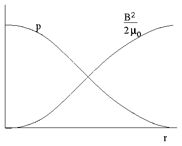
Figure 4.7: Balance of kinetic and magnetic pressure
|
|
Bz2
2 μo
|
+ p = |
Bz ext2
2 μo
|
|
| (4.126) |
[Recall Single Particle Problem]
Think of these as a pressure equation. Equilibrium says total
pressure = const.
|
|
magnetic pressure
|
+ |
p
kinetic pressure
|
= const. |
| (4.127) |
Ratio of kinetic to magnetic pressure is plasma `β'.
measures `efficiency' of plasma confinement by B.
Want large β for fusion but limited by instabilities, etc.
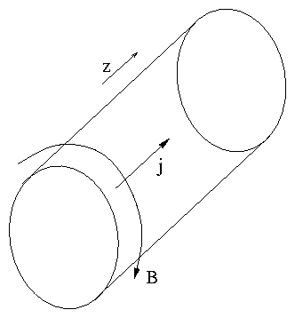
4.8.2 Z-pinch
Figure 4.8: Z-pinch configuration.
so called because j flows in z-direction.
Again take to be ∞ length and uniform.
|
j = jz |
^
e
|
z
|
B
= Bθ |
^
e
|
θ
|
|
| (4.129) |
|
Force ( j ∧B)r − ( ∇p )r = − jz Bθ − |
∂p
∂r
|
= 0 |
| (4.130) |
|
Ampere ( ∇ ∧B)z − ( μo j )z = |
1
r
|
|
∂
∂r
|
( r Bθ ) − μojz = 0 |
| (4.131) |
Eliminate j:
|
|
Bθ
μo r
|
|
∂
∂r
|
( r Bθ ) + |
∂p
∂r
|
= 0 |
| (4.132) |
or
|
|
Extra Term
|
+ |
∂
∂r
|
|
Magnetic + Kinetic pressure
|
= 0 |
| (4.133) |
Extra term acts like a magnetic tension force. Arises because
B-field lines are curved.
Can integrate equation
|
| ⌠
⌡
|
b
a
|
|
Bθ2
μo
|
|
dr
r
|
+ | ⎡
⎣
|
Bθ2
2 μo
|
+ p(r) | ⎤
⎦
|
b
a
|
= 0 |
| (4.134) |
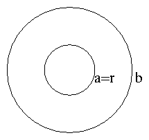
If we choose b to be edge (p(b)=0) and set a=r we get
Figure 4.9: Radii of integration limits.
|
p(r) = |
Bθ2 ( b )
2 μo
|
− |
Bθ2 ( r )
2 μo
|
+ | ⌠
⌡
|
b
r
|
|
Bθ2
μo
|
|
dr′
r′
|
|
| (4.135) |
Force balance in z-pinch is somewhat more complicated because
of the tension force. We can't choose p(r) and j(r)
independently; they have to be self consistent.
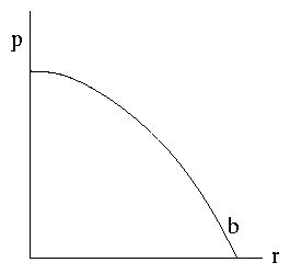
Example j = const.
|
|
1
r
|
|
∂
∂r
|
( r Bθ ) = μo jz ⇒ Bθ = |
μo jz
2
|
r |
| (4.136) |
Hence
| |
|
|
|
1
2 μo
|
| ⎛
⎝
|
μo jz
2
| ⎞
⎠
|
2
|
{ b2 − r2 + | ⌠
⌡
|
b
r
|
2 r′dr′} |
| | (4.137) |
| |
|
| | (4.138) |
|
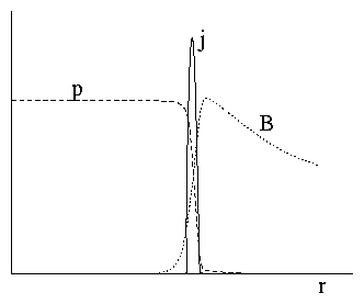
Figure 4.10: Parabolic Pressure Profile.
Also note Bθ (b) = [( μo jzb)/2] so
|
p = |
Bθb2
2 μo
|
|
2
b2
|
{ b2 − r2 } |
| (4.139) |
4.8.3 `Stabilized Z-pinch'
Also called `screw pinch', θ−z pinch or sometimes
loosely just `z-pinch'.
Z-pinch with some additional Bz as well as
Bθ
|
(Force)r jθ Bz − jz Bθ − |
∂p
∂r
|
= 0 |
| (4.140) |
|
|
1
r
|
|
∂
∂r
|
( r Bθ ) = μo jz |
| (4.142) |
Eliminate j:
|
− |
Bz
μo
|
|
∂Bz
∂r
|
− |
Bθ
μo r
|
|
∂
∂r
|
( r Bθ ) − |
∂p
∂r
|
= 0 |
| (4.143) |
or
|
|
[(Mag Tension) || (θ only)]
|
+ |
∂
∂r
|
|
Mag (θ+z) + Kinetic pressure
|
= 0 |
| (4.144) |
4.9 Some General Properties of MHD Equilibria
4.9.1 Pressure & Tension
|
j ∧B− ∇p = 0 : ∇ ∧B
= μo j |
| (4.145) |
We can eliminate j in the general case
to get
Expand the vector triple product:
|
∇p = |
1
μo
|
( B. ∇ )B− |
1
2 μo
|
∇ B2 |
| (4.147) |
put b = [(B)/ | B | ] so that
∇B
= ∇(B b) = B ∇b + b ∇B.
Then
| |
|
|
|
1
μo
|
{ B2 ( b . ∇ ) b + B b ( b . ∇ ) B } − |
1
2 μo
|
∇ B2 |
| | (4.148) |
| |
|
|
|
B2
μo
|
( b . ∇ )b − |
1
2 μo
|
( ∇ − b ( b . ∇ ) ) B2 |
| | (4.149) |
| |
|
|
B2
μo
|
( b . ∇ ) b − ∇⊥ | ⎛
⎝
|
B2
2 μ0
| ⎞
⎠
|
|
| | (4.150) |
|
Now ∇⊥ ( [(B2)/(2 μo)] ) is the
perpendicular (to B) derivative of magnetic pressure
and (b . ∇)b is the
curvature of the magnetic field line giving
tension.
| ( b .∇ ) b | has value
1/R.
R: radius of curvature.
4.9.2 Magnetic Surfaces
|
0 = B. [ j ∧B− ∇p ] = − B. ∇ p |
| (4.151) |
*Pressure is constant on a field line (in MHD situation).
(Similarly, 0 = j . [ j ∧B− ∇p ] = j . ∇ p.)
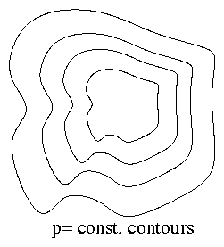
Figure 4.11: Contours of pressure.
Consider some arbitrary
volume in which ∇p ≠ 0. That is, some
plasma of whatever shape. Draw contours (surfaces in
3-d) on which p = const. At any point on such an
isobaric surface ∇p is perp to the surface.
But B. ∇ p = 0 implies that B is
also perp to ∇p.
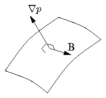
Figure 4.12: B is perpendicular to ∇p
and so lies in the isobaric surface.
Hence
B lies in the surface p = const.
In equilibrium isobaric surfaces are
`magnetic surfaces'.
[This argument does not work if p = const. i.e.
∇ p = 0. Then there need be no magnetic
surfaces.]
4.9.3 `Current Surfaces'
Since j . ∇ p = 0 in equilibrium the
same argument applies to current density. That is
j lies in the surface p = const.
Isobaric Surfaces are `Current Surfaces'.
Moreover it is clear that
`Magnetic Surfaces' are `Current Surfaces'.
(since both coincide with isobaric surfaces.)
[It is important to note that the existence of magnetic
surfaces is guaranteed only in the MHD approximation when
∇p ≠ 0 Taking account of corrections to
MHD we may not have magnetic surfaces even if ∇p ≠ 0.]
4.9.4 Low β equilibria: Force-Free Plasmas
In many cases the ratio of kinetic to magnetic pressure is
small, β << 1 and we can approximately ignore
∇p. Such an equilibrium is called `force free'.
implies j and B are parallel.
i.e.
Current flows along field lines not across.
Take divergence:
| |
|
|
∇ . j = ∇ . ( μ( r ) B) = μ( r ) ∇ . B+ ( B. ∇ ) μ |
| | (4.154) |
| |
|
| | (4.155) |
|
The ratio j/B = μ is constant along field lines.
μ is constant on a magnetic surface. If there are no surfaces,
μ is constant everywhere.
Example: Force-Free Cylindrical Equil.
This is a somewhat more convenient form because it is linear
in B (for specified μ(r)).
leads to a Bessel function solution
for μo μr > 1st zero of J0 the
toroidal field reverses. There are plasma
confinement schemes with μ ≅ const.
`Reversed Field Pinch'.
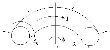
4.10 Toroidal Equilibrium
Bend a z-pinch into a torus
Figure 4.13: Toroidal z-pinch
Bθ fields due to current are stronger at small
R side ⇒ Pressure (Magnetic) Force
outwards.
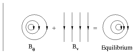
Have to balance this by applying a vertical field Bv
to push plasma back by jϕ ∧Bv.
Figure 4.14: The field of a toroidal
loop is not an MHD equilibrium. Need to add a vertical field.
Bend a θ-pinch into a torus:
Bϕ is stronger at small R side
⇒ outward force.
Cannot be balanced by Bv because no
jϕ.
No equilibrium for a toroidally symmetric θ-pinch.
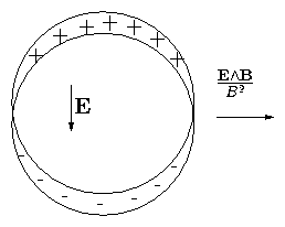
Underlying Single Particle reason:
Toroidal θ-pinch has Bϕ only. As we have
seen before, curvature drifts are uncompensated in such a
configuration and lead to rapid outward
motion.
Figure 4.15: Charge-separation giving outward
drift is equivalent to the lack of MHD toroidal force balance.
We know how to solve this: Rotational Transform:
get some Bθ. Easiest way: add jϕ.
From MHD viewpoint this allows you to push the plasma
back by jϕ ∧Bv force. Essentially,
this is Tokamak.
4.11 Plasma Dynamics (MHD)
When we want to analyze non-equilibrium situations
we must retain the momentum terms. This will give a dynamic
problem. Before doing this, though, let us analyse some
purely Kinematic Effects.
`Ideal MHD' ⇔ Set η = 0 in Ohm's Law.
A good approximation for high frequencies, i.e. times shorter
than resistive decay time.
|
E+ V ∧B= 0 . Ideal Ohm′s Law. |
| (4.161) |
Also
|
∇ ∧E= |
− ∂B
∂t
|
Faraday′s Law. |
| (4.162) |
Together these two equations imply constraints on how the magnetic
field can change with time: Eliminate E:
This shows that the changes in B are completely determined
by the flow, V.
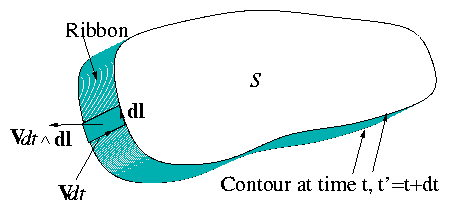
4.12 Flux Conservation
Consider an arbitrary closed contour C and spanning surface
S in the fluid.
Flux linked by C is
Let C and S move with fluid:
Figure 4.16: Motion of contour with fluid gives
convective flux derivative term.
Total rate of change of Φ is given by two terms:
| |
|
|
| ⌠
⌡
|
S
|
|
Due to changes in B
|
+ |
Due to motion of C
|
|
| | (4.165) |
| |
|
|
− | ⌠
⌡
|
S
|
∇ ∧E. ds − | ⌠
(⎜)
⌡
|
C
|
( V ∧B) . d l |
| | (4.166) |
| |
|
| − | ⌠
(⎜)
⌡
|
C
|
(E+ V ∧B) . d l = 0 by Ideal Ohm′s Law. |
| | (4.167) |
|
Flux through any surface moving with fluid is conserved.
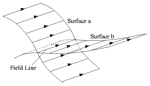
4.13 Field Line Motion
Figure 4.17: Field line defined by intersection
of two flux surfaces tangential to field.
Think of a field line as the intersection of two surfaces
both tangential to the field everywhere:
Let surfaces move with fluid.
Since all parts of surfaces had zero flux crossing at
start, they also have zero after, (by flux conservation).
That means their surfaces are tangent also after motion.
Hence their intersection defines a field line after the motion.
We think of the new field line as the same line as the old
one (only moved).
Thus:
- Number of field lines ( ≡ flux) through any
surface is constant. (Flux Cons.)
- A line of fluid that starts as a field line remains
one. Frozen-in field lines.
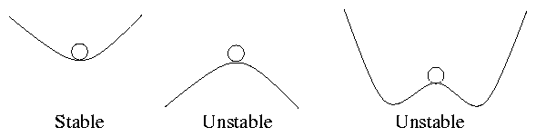
4.14 MHD Stability
The fact that one can find an MHD equilibrium
(e.g. z-pinch) does not guarantee a useful confinement
scheme because the equil. might be unstable. Ball on hill
analogies:
Figure 4.18: Potential energy curves
An equilibrium is unstable if the curvature of the
`Potential energy surface' is downward away from equil.
That is if [( d2)/(dx2)] { Wpot } < 0.
In MHD the potential energy is Magnetic + Kinetic Pressure
(usually mostly magnetic).
If we can find any type of perturbation which lowers
the potential energy then the equil is unstable. It will
not remain but will rapidly be lost.
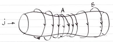
Example Z-pinch
We know that there is an equilibrium: Is it stable?
Consider a perturbation thus:
Figure 4.19: 'Sausage' instability
Simplify the picture by taking the current all to flow in a
skin. We know that the pressure is supported by the combination
of B2/2 μo pressure and
[(B2)/(μor)] tension forces.
Figure 4.20: Skin-current, sharp boundary pinch.
At the place where it pinches in (A)
Bθ and 1/r increase ⇒ Magnetic
pressure & tension increase, ⇒ inward force
no longer balanced by p, ⇒ perturbation grows.
At place where it bulges out (B)
Bθ & 1/r decrease ⇒
Magnetic pressure & tension decrease ⇒ perturbation grows.
Conclusion a small perturbation induces a small force imbalance
tending to increase the perturbation. That means it is Unstable
( ≡ δW < 0).
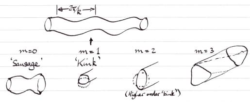
4.15 General Perturbations of Cylindrical Equil.
Look for things which go like exp[i(kz + mθ)].
[Fourier (Normal Mode) Analysis].
Figure 4.21: Types of kink perturbation.
Generally Helical in form (like a screw thread).
Example: m=1 k ≠ 0 z-pinch
Figure 4.22: Driving force of a kink. Net force
tends to increase perturbation. Unstable.
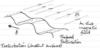
4.16 General Principles Governing Instabilities
(1) They try not to bend field lines. (Because bending takes
energy; think of a stretched elastic string). Not bending field lines
requires perturbation (Constant surfaces) to lie along magnetic
field.
Figure 4.23: Alignment of perturbation and field
line minimizes bending energy.
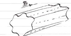
Example: θ-pinch type plasma column:
Figure 4.24: `Flute' or `Interchange' modes.
Preferred Perturbations are `Flutes' as per Greek columns
→ `Flute Instability.' [Better name:
`Interchange Instability', arises from idea that plasma
and vacuum change places.]
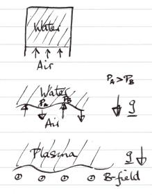
(2) Occur when a `heavier' fluid is supported by a `lighter'
(Gravitational analogy). See Fig. 4.25.
Figure 4.25: Inverted water glass analogy. Rayleigh
Taylor instability.
Why does water fall out of an inverted glass?
Air pressure could sustain it but does not because
of Rayleigh-Taylor instability.
Similar for supporting a plasma by mag field.
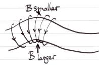
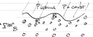
(3) Occur when | B | decreases away
from the plasma region. See Fig. 4.26.
Figure 4.26: Vertical upward field gradient is
unstable.
⇒ Perturbation Grows.
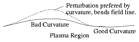
(4) Occur when field line curvature is towards
the plasma (Equivalent to (3) because of ∇ ∧B
= 0 in a vacuum).
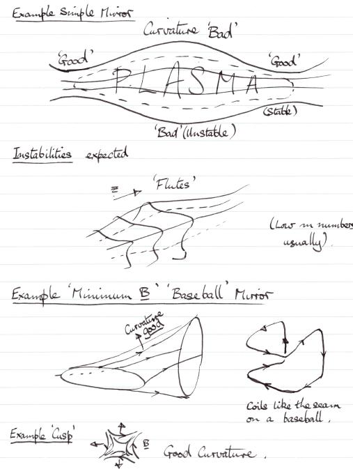
Figure 4.27: Examples of magnetic configurations with good and bad curvature.
4.17 Quick and Simple Analysis of Pinches
θ-pinch | B | = const. outside pinch
≡ No field line curvature. Neutral stability
z-pinch ∇ | B | away from plasma outside
≡ Bad Curvature (Towards plasma) ⇒
Instability.
Generally it is difficult to get the curvature to be good everywhere.
Often it is sufficient to make it good on average on a field
line. This is referred to as `Average Minimum B'. Tokamak has this.
General idea is that if field line is only in bad curvature over part
of its length then to perturb in that region and not in the good
region requires field line bending:
Figure 4.28: Parallel localization of perturbation
requires bending.
But bending is not preferred. So this may stabilize.
Possible way to stabilize configuration with bad
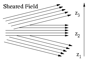
curvature: Shear
Shear of Field Lines
Figure 4.29: Depiction of field shear.
Direction of B changes. A perturbation along B at z3 is
not along B at z2 or z1 so it would have to
bend field there → Stabilizing effect.
General Principle: Field line bending is stabilizing.
Example: Stabilized z-pinch
Perturbations (e.g. sausage or kink) bend
Bz so the tension in Bz acts as a restoring force
to prevent instability. If wave length very long
bending is less. ⇒ Least stable tends to be
longest wave length.
Example: `Cylindrical Tokamak'
Tokamak is in some ways like a periodic cylindrical stabilized
pinch. Longest allowable wave length = 1 turn round torus
the long way, i.e.
Express this in terms of a toroidal mode number, n
(s.t. perturbation ∝ expi (nϕ+ mθ):
ϕ = z/R n = kR.
Most unstable mode tends to be n=1.
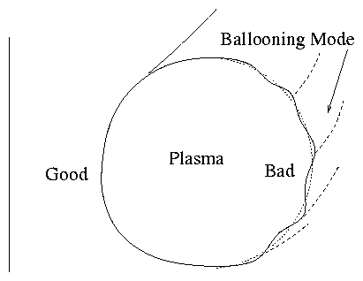
[Careful! Tokamak has important toroidal effects and some
modes can be localized in the bad curvature region
(n ≠ 1).
Figure 4.30: Ballooning modes are localized in the
outboard, bad curvature region.
4.18 Rayleigh Taylor Instability Analysis
Here we give an elementary mathematical derivation of the (in)stability
criterion for a fluid supported against gravity and show that it is
equivalent to a plasma under the influence of curvature
forces. Although the treatment is general, rigor is sacrificed in the
interests of brevity and clarity,
Consider a simple fluid (air, water, whatever). Its momentum equation
is
|
ρ | ⎛
⎝
|
∂
∂t
|
+ v.∇ | ⎞
⎠
|
v = −∇p + ρg, |
| (4.170) |
where g is the gravity force vector pointing in the
-z-direction. If the fluid starts at rest, then the term
v.∇v is second order and ignorable in the linearized analysis
we do.
We take the curl of the momentum equation (to annihilate ∇p)
and get
|
∇∧ρ |
∂v
∂t
|
=∇∧ρg ( = ∇ρ∧g) |
| (4.171) |
We write the equilibrium quantities as e.g. ρ0, and look for
first-order perturbed quantities (e.g. ρ1) that vary like
exp(ik.x), where k is perpendicular to ∧z. One can show
that the most unstable motions are displacements ξ that are in
the vertical z-direction, so that k.v
=0 and the flow is
incompressible. Obviously, also v
=∂ξ/∂t. The
first order terms of eq. (4.171) are then
|
∇∧ | ⎛
⎝
|
ρ0 |
∂2 ξ
∂t2
|
− gρ1 | ⎞
⎠
|
=0. |
| (4.172) |
Using ξ's incompressibility in the continuity equation we find,
and when substituted into eq. (4.172) we get
|
∇∧ | ⎛
⎝
|
ρ0 |
∂2 ξ
∂t2
|
+ ξ |
∂ρ0
∂z
|
g | ⎞
⎠
|
=0. |
| (4.174) |
This equation is satisfied (only) by setting the bracket equal to
zero, and noting that since its vectors (ξ
=ξ∧z,
g
=−g∧z) both point in the ∧z direction it is effectively a
scalar equation
|
|
∂2 ξ
∂t2
|
= | ⎛
⎝
|
g
ρ0
|
|
∂ρ0
∂z
| ⎞
⎠
|
ξ. |
| (4.175) |
The solutions of this equation grow exponentially (unstably), with
growth rate
γ = √{[g/(ρ0)][(∂ρ0)/(∂z)]}, if
([g/(ρ0)][(∂ρ0)/(∂z)]) > 0.
They are instead are purely oscillatory (stable) if
([g/(ρ0)][(∂ρ0)/(∂z)]) < 0. The
criterion for instability, which can be written more formally as
g.∇ρ0 < 0, can be thought of informally as saying "a lower
density (lighter) fluid supported by a higher density (heavier) fluid
is unstable". All of this is for neutral fluids, the instability is
called Rayleigh-Taylor.
MHD plasma stability. Magnetic Field with gravity
The momentum equation can be written
|
ρ | ⎛
⎝
|
∂
∂t
|
+ v.∇ | ⎞
⎠
|
v = −∇ | ⎛
⎝
|
p + |
B2
2μ0
| ⎞
⎠
|
+ |
1
μ0
|
(B.∇)B+ ρg, |
| (4.176) |
If the term (B.∇)B were ignorable (and the directions of g
and ∇ρ0 coincide and are perpendicular to B) the
analysis would be identical. That term (B.∇)B has two
possible first order parts: (B0.ik)B1 and (B1.∇)B0, I
will concentrate only on the first, and ignore the second because for
an equilibrium uniform perpendicular to ∧g, with B0
perpendicular to ∧g, the second has zero ∧g component. Now
(B0.ik)B1 is zero if B0.k
=0, that is, if the perturbation
wave-fronts are field-aligned. Nothing then stabilizes the
Rayleigh-Taylor instability if g.∇ρ0 < 0, and the prior
analysis applies. If, however, the term (B0.ik) B1 is not zero, then
|
∇∧ | ⎡
⎣
|
ρ0 |
∂2 ξ
∂t2
|
+ ξg.∇ρ0 −(B0.ik)B1/μ0 | ⎤
⎦
|
=0. |
| (4.177) |
The ∧g-component (formerly the z-component) of B1 must be
considered. By the freezing in of field-lines, and simple geometry,
|
B1g = B0.∇ξg = i(B0.k)ξg. |
| (4.178) |
Therefore the scalar equation that must be satisfied is
|
− |
∂2 ξ
∂t2
|
= |
1
ρ0
|
[g.∇ρ0+(B0.k)2/μ0]ξ. |
| (4.179) |
The magnetic term is always positive, which is stabilizing. If
(B0.k)2 > −g.∇(ρ0), then the mode is stable
(oscillatory). Otherwise the destabilizing g-term overcomes the
stabilizing bending term.
Equivalence of Field-Curvature and Gravity
Consider a vacuum field for simplicity (this can be generalized); the
combined grad-B and curvature drift is
|
vd=(mv⊥2/2 + mv||2) |
Rc∧B
qRc2B2
|
, |
| (4.180) |
which can be considered to arise from the generalized force expression
with the centrifugal and −μ∇B forces. By simple inspection
of the above equation, the force per particle giving rise to it is
(mv⊥2/2 + mv||2)Rc/Rc2. Averaged over a
Maxwellian distribution, both the energy terms are T, so the force
density is
|
Fc = 2nTRc/Rc2 = 2pRc/Rc2. |
| (4.181) |
This is the quantity that is equivalent to ρ0g. It points in
the direction of the radius of curvature Rc. If ∇.Fc < 0,
then the plasma is unstable to perturbations for which k.B0=0.
Substituting for Fc, the more general instability criterion for
non-field-aligned perturbations is
|
(Rc.∇p)/Rc2 < (B0.k)2/2μ0. |
| (4.182) |
Then we think of ∇p as being "inward", toward
the hot dense center of a confined plasma. In which case the radius
curvature being "outward" is unfavorable for stability.
[It might seem that since we always need the most unstable mode, the
stabilizing effects of B0.k are irrelevant because the most
unstable mode will always choose this to be zero. However, if field
has shear then as soon as one moves away (in the ∧g
direction) from the place where B0.k
=0 has been chosen, the field
angle changes; so B0.k is no longer zero. Consequently, there
will be a trade-off between localization of the eigenmode in the
∧g-direction which implies compression, and field line
bending. Also, sometimes Fc can vary from stabilizing to
destabilizing along the field; then no perturbation that zeroes
B0.k everywhere can be localized to where Fc is destabilizing.]