Chapter 1
Fitting Functions to Data
1.1 Exact fitting
1.1.1 Introduction
Suppose we have a set of real-number data pairs xi,yi, i=1,2,... N. These can be considered to be a set of points in the
xy-plane. They can also be thought of as a set of values y of a
function of x; see Fig. 1.1.
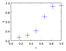
Figure 1.1: Example of data to be fitted with a curve.
|
f(xi)=yi, for all i=1,...,N. |
| (1.1) |
When the number of pairs is small and they are reasonably spaced out
in x, then it may be reasonable to do an exact fit that satisfies this
equation.
1.1.2 Representing an exact fitting function linearly
We have an infinite choice of possible fitting functions. Those functions must have a number of different adjustable
parameters that are set so as to adjust the function to fit the
data. One example is a polynomial.
|
f(x) = c1 + c2 x + c3 x2 + ... + cN xN−1 |
| (1.2) |
Here the ci are the coefficients that must be adjusted to make the
function fit the data. A polynomial whose coefficients are the
adjustable parameters has a very useful property that it is linearly
dependent upon the coefficients.
In order to fit eqs. (1.1) with the form of eq. (1.2)
requires that N simultaneous equations be satisfied. Those equations
can be written as an N×N matrix equation as
follows:
|
| ⎛
⎜
⎜
⎜
⎜
⎜
⎝
|
| ⎞
⎟
⎟
⎟
⎟
⎟
⎠
|
| ⎛
⎜
⎜
⎜
⎜
⎜
⎝
|
| ⎞
⎟
⎟
⎟
⎟
⎟
⎠
|
= | ⎛
⎜
⎜
⎜
⎜
⎜
⎝
|
| ⎞
⎟
⎟
⎟
⎟
⎟
⎠
|
|
| (1.3) |
Here we notice that in order for this to be a square matrix system we
need the number of coefficients to be equal to the number of data
pairs, N.
We also see that we could have used any set of N functions fi as
fitting functions, and written the representation:
|
f(x) = c1f1(x) + c2 f2(x) + c3 f3(x) + ... + cN fN(x) |
| (1.4) |
and then we would have obtained the matrix equation
|
| ⎛
⎜
⎜
⎜
⎜
⎜
⎝
|
| ⎞
⎟
⎟
⎟
⎟
⎟
⎠
|
| ⎛
⎜
⎜
⎜
⎜
⎜
⎝
|
| ⎞
⎟
⎟
⎟
⎟
⎟
⎠
|
= | ⎛
⎜
⎜
⎜
⎜
⎜
⎝
|
| ⎞
⎟
⎟
⎟
⎟
⎟
⎠
|
|
| (1.5) |
This is the most general form of representation of a fitting
function that varies linearly with the unknown coefficients. The
matrix1 we will call S. It has elements Sij=fj(xi)
1.1.3 Solving for the coefficients
When we have a matrix equation of the form
Sc = y, where S is a square matrix, then provided
that the matrix is non-singular, that is, provided its
determinant is
non-zero, |S| ≠ 0, it possesses an inverse S−1. Multiplying on the left by this inverse we
get:
In other words, we can solve for c, the unknown coefficients,
by inverting the function matrix, and multiplying the values to be
fitted, y by that inverse.
Once we have the values of c we can evaluate the function
f(x)
(eq. 1.2) at any x-value we like.
Fig. 1.2 shows the result of fitting a 5th order
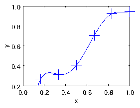
Figure 1.2: Result of the polynomial fit.
1.2 Approximate Fitting
If we have lots of data which has scatter in it, arising from
uncertainties or noise, then we almost certainly
do not want to fit a curve so that it goes exactly through
every point. For example see Fig. 1.3.
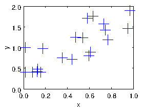
Figure 1.3: A cloud of points with uncertainties and noise, to be fitted
with a function.
|
f(x) = c1f1(x) + c2 f2(x) + c3 f3(x) + ... + cM fM(x) |
| (1.7) |
in which usually M < N. We know now that we can't fit the data
exactly. The set of equations we would have to satisfy to do so would
be
|
| ⎛
⎜
⎜
⎜
⎜
⎜
⎝
|
| ⎞
⎟
⎟
⎟
⎟
⎟
⎠
|
| ⎛
⎜
⎜
⎜
⎜
⎜
⎝
|
| ⎞
⎟
⎟
⎟
⎟
⎟
⎠
|
= | ⎛
⎜
⎜
⎜
⎜
⎜
⎝
|
| ⎞
⎟
⎟
⎟
⎟
⎟
⎠
|
|
| (1.8) |
in which the function matrix S is now not square but has
dimensions N×M. There are not enough coefficients cj to be
able to satisfy these equations exactly. They are
over-specified. Moreover, a non-square matrix doesn't have an inverse.
But we are not interested in fitting this data exactly. We want to fit
some sort of line through the points that best-fits them.
1.2.1 Linear Least Squares
What do we mean by "best fit"?
Especially when fitting a function of the linear form eq. (1.7), we usually mean that we want to minimize the vertical
distance between the points and the line. If we had a fitted function
f(x), then for each data pair (xi,yi), the square of the
vertical distance between the line and the point is
(yi−f(xi))2. So the sum, over all the points, of the square
distance from the line is
|
χ2 = |
∑
i=1,N
|
(yi−f(xi))2 . |
| (1.9) |
We use the square of the distances in part because they are
always positive. We don't want to add positive and negative distances,
because a negative distance is just as bad as a positive one and we
don't want them to cancel out.
We generally call χ2 the "residual", or more simply
the "chi-squared". It is an inverse measure of
goodness of fit. The smaller it is the better. A linear least squares
problem is: find the coefficients of our function f that minimize
the residual χ2.
1.2.2 SVD and the Moore-Penrose Pseudo-inverse
We seem to have gone off in a different direction from our original
way to solve for the fitting coefficients by inverting the square
matrix S. How is that related to the finding of the
least-squares solution to the over-specified set of equations (1.8)?
The answer is a piece of matrix magic! It turns out that there
is (contrary to what one is taught in an elementary matrix
course) a way to define the inverse of a non-square matrix or of a
singular square matrix. It is called the (Moore-Penrose) pseudo-inverse.
And once found it can be used in essentially exactly the way we did for the
non-singular square matrix in the earlier treatment. That is, we solve
for the coefficients using c = S−1 y, except
that S−1 is now the pseudo-inverse.
The pseudo-inverse is best understood from a consideration of what is
called the Singular Value Decomposition (SVD) of a matrix. This is the
embodiment of a theorem in matrix mathematics that states that any
N×M matrix can always be expressed as the product
of three other matrices with very special properties. For our N×M matrix S this expression is:
where T denotes transpose, and
- U is an N×N orthonormal matrix
- V is an M×M orthonormal matrix
- D is an N×M diagonal matrix
Orthonormal3 means that the dot product of any
column (regarded as a vector) with any other column is zero, and the
dot product of a column with itself is unity. The inverse of an
orthonormal matrix is its transpose. So
|
|
UT
N×N
|
|
U
N×N
|
= |
I
N×N
|
and |
VT
M×M
|
|
V
M×M
|
= |
I
M×M
|
|
| (1.11) |
A diagonal matrix has
non-zero elements only on the diagonal. But if it is non-square, as it
is if M < N, then it is padded with extra rows of zeros (or extra
columns if N < M).
|
D = | ⎛
⎜
⎜
⎜
⎜
⎜
⎜
⎜
⎝
|
| ⎞
⎟
⎟
⎟
⎟
⎟
⎟
⎟
⎠
|
|
| (1.12) |
A sense of what the SVD is can be gained from by thinking4 in terms of the
eigenanalysis of the matrix
STS. Its eigenvalues are di2.
The pseudo-inverse can be considered to be
Here D−1 is a M×N diagonal matrix whose entries are
the inverse of those of D, i.e. 1/dj:
|
D−1 = | ⎛
⎜
⎜
⎜
⎜
⎜
⎜
⎝
|
| ⎞
⎟
⎟
⎟
⎟
⎟
⎟
⎠
|
. |
| (1.14) |
It's clear that eq. (1.13)
is in some sense an inverse of S, because formally
|
S−1 S = (VD−1UT)( UDVT) = VD−1DVT = VVT = I . |
| (1.15) |
If M ≤ N and none of the dj is zero, then all the
operations in this matrix multiplication reduction are valid, because
But see the enrichment section5 for detailed discussion
of other cases.
The most important thing for our present purposes is that if M ≤ N
then we can find a solution of the over-specified (rectangular matrix)
fitting problem Sc = y as
c=S−1y, using the pseudo-inverse. The set of
coefficients c we get corresponds to more than one possible
set of yi-values, but that does not matter.
Also, one can show6, that the specific solution that is obtained by this
matrix product is in fact the least squares solution for
c; i.e. the solution that minimizes the residual
χ2. And if there is any freedom in the choice of c, such
that the residual is at its minimum for a range of different
c, then the solution which minimizes |c|2 is the one
found.
The beauty of this fact is that one can implement a simple code, which
calls a function pinv to find the
pseudo-inverse, and it will work just fine if
the matrix S is singular or even rectangular.
As a matter of computational efficiency, one should note that in
Octave the backslash operator,
is equivalent to multiplying by the pseudo-inverse
(i.e. pinv(S)*y = S\y), but calculated far more efficiently7. So backslash is
preferable in computationally costly code, because it is roughly 5
times faster. You probably won't notice the difference for matrix
dimensions smaller than a few hundred.
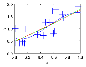
Figure 1.4: The cloud of points fitted with linear, quadratic, and cubic
polynomials.
1.2.3 Smoothing and Regularization
As we illustrate in Fig. 1.4, by choosing the number of degrees of
freedom of the fitting function one can
adjust the smoothness of the fit to the data. However, the choice of
basis functions then constrains one in a way
that has been pre-specified. It might not in fact be the best way to
smooth the data to fit it by (say) a straight line or a parabola.
A better way to smooth is by "regularization" in which we add some
measure of roughness to the residual we are seeking
to minimize. The roughness (which is the inverse of the smoothness) is
a measure of how wiggly the fit line is. It can in principle be pretty
much anything that can be written in the form of a matrix times the
fit coefficients. I'll give an example in a moment. Let's assume the
roughness measure is homogeneous, in the sense that we are trying to
make it as near zero as possible. Such a target would be Rc = 0, where R is a matrix of dimension NR×M,
where NR is the number of distinct roughness
constraints. Presumably we can't satisfy this equation perfectly
because a fully smooth function would have no variation, and be unable
to fit the data. But we want to minimize the square of the roughness
(Rc)TR c. We can try to fulfil the
requirement to fit the data, and to minimize the roughness, in a
least-squares sense by constructing an expanded compound matrix system
combining the original equations and the regularization,
thus8
|
| ⎛
⎜
⎜
⎝
|
| ⎞
⎟
⎟
⎠
|
c = | ⎛
⎜
⎜
⎝
|
| ⎞
⎟
⎟
⎠
|
. |
| (1.17) |
If we solve this system in a least-squares sense by using the pseudo
inverse of the compound matrix
, then we will have found the coefficients
that "best" make the roughness zero as well as fitting the data: in
the sense that the total residual
|
χ2 = |
∑
i=1,N
|
(yi−f(xi))2 + λ2 |
∑
k=1,NR
|
( |
∑
j
|
Rkjcj)2 |
| (1.18) |
is minimized. The value of λ controls the weight of the
smoothing. If it is large, then we prefer smoother solutions. If it is
small or zero we do negligible smoothing.
As a specific one-dimensional example, we might decide that the
roughness we want to minimize is represented by the second derivative
of the function: d2f/dx2. Making this quantity on average small
has the effect of minimizing the wiggles in the function, so it is an
appropriate roughness measure. We could therefore choose R such that it
represented that derivative at a set of chosen points xk, k=1,NR
(not the same as the data points xi) in which case:
The xk might, for example, be equally spaced over the x-interval
of interest, in which case9 the squared roughness measure could be
considered a discrete approximation to the integral, over the interval, of
the quantity (d2f/dx2)2.
1.3 Tomographic Image Reconstruction
Consider the problem of x-ray tomography. We make many measurements of
the integrated density of matter along chords in a plane section
through some object whose interior we wish to reconstruct. These are
generally done by measuring the attenuation of x-rays
along each chord, but the mathematical technique is independent of the
physics. We seek a representation of the density of the
object in the form
|
ρ(x,y) = |
∑
j=1,M
|
cj ρj(x,y), |
| (1.20) |
where ρj(x,y) are basis functions over the
plane. They might actually be as simple as
pixels over mesh xk and yl, such that
ρj(x,y)→ ρkl(x,y) = 1 when xk < x < xk+1 and
yl < y < yl+1, and zero otherwise. However, the form of basis
function that won Alan Cormack the Nobel
prize for medicine in his implementation of "computerized tomography"
(the CT scan) was much more
cleverly chosen to build the smoothing into the basis functions. Be
careful thinking about multidimensional fitting. For constructing
fitting matrices, the list of basis functions should be considered to
be logically arranged from 1 to M in a single index j so that the
coefficients are a single column vector. But the physical arrangement
of the basis functions might more naturally be expressed using two
indices k,l referring to the different spatial dimensions. If so
then they must be mapped in some consistent manner to the vector
column.
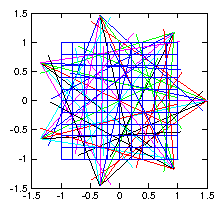
Figure 1.5: Illustrative layout of
tomographic reconstruction of density in a plane
using multiple fans of chordal observations.
Each chord along which measurements are made, passes through the basis
functions (e.g. the pixels), and for a particular set of coefficients
cj we therefore get a chordal measurement value
|
vi = | ⌠
⌡
|
li
|
ρdl = | ⌠
⌡
|
li
|
|
∑
j=1,M
|
cj ρj(x,y) dl = |
∑
j=1,M
|
| ⌠
⌡
|
li
|
ρj(x,y) dl cj = Sc, |
| (1.21) |
where the N×M matrix S is formed from the integrals
along each of the N lines of sight li, so that
Sij=∫li ρj(x,y) dl. It represents the contribution of
basis function j to measurement i. Our fitting problem is thus
rendered into the standard form:
in which a rather large number M of basis functions might be involved.
We can solve this by pseudo-inverse:
c=S−1v, and if the system is overdetermined,
such that the effective number of different chords is larger than the
number of basis functions, it will probably work.
The problem is, however, usually
under-determined, in the sense that we
don't really have enough independent chordal measurements to determine
the density in each pixel (for example). This is true even if we
apparently have more measurements than pixels, because generally there
is a finite noise or uncertainty level in the chordal measurements
that becomes amplified by the inversion process. This is illustrated
by a simple test as shown in Fig. 1.6.
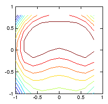
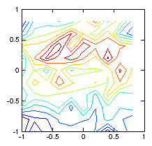
Figure 1.6: Contour plots of the initial test ρ-function (left) used to
calculate the chordal integrals, and its reconstruction based upon
inversion of the chordal data (right). The number of pixels (100)
exceeds the number of views (49), and the number of singular
values used in the pseudo inverse is restricted to 30. Still they
do not agree well, because various artifacts appear. Reducing the
number of singular values does not help.
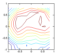
Figure 1.7: Reconstruction using a regularization smoothing based upon
∇
2ρ. The contours are much nearer to reality.
1.4 Efficiency and Nonlinearity
Using the inverse or
pseudo-inverse to solve for the coefficients of a fitting function is
intuitive and straight-forward. However, in many cases it is
not the most computationally efficient approach. For moderate
size problems, modern computers have more than enough power to
overcome the inefficiencies, but in a situation with multiple
dimensions, such as tomography, it is easy for the matrix that needs
to be inverted to become enormous, because that matrix's side length
is the total number of pixels or elements in the fit, which may
be, for example, the product of the side lengths
nx×ny. The giant matrix that has to be inverted,
may be very "sparse", meaning
that all but a very few of its elements are zero. It can then become
overwhelming in terms of storage and cpu to use the direct inversion
methods we have discussed here. We'll see other approaches later.
Some fitting problems are
nonlinear. For example,
suppose one had a photon spectrum of a
particular spectral line to which one wished to fit a
Gaussian function of particular
center, width, and height. That's a problem that cannot be expressed
as a linear sum of functions. In that case fitting becomes more
elaborate10, and less
reliable. There are some potted fitting programs out there, but it's
usually better if you can avoid them.
Worked Example: Fitting sinusoidal functions
Suppose we wish to fit a set of data xi,yi spread over the range
of independent variable a ≤ x ≤ b. And suppose we know the
function is zero at the boundaries of the range, at x=a and
x=b. It makes sense to incorporate our
knowledge of the boundary values into the
choice of functions to fit, and choose those functions fn to be
zero at x=a and x=b. There are numerous well known sets of
functions that have the property of being zero at two separated
points. The points where standard functions are zero are of course not
some arbitrary a and b. But we can scale the independent variable
x so that a and b are mapped to the appropriate points for any
choice of function set.
Suppose the functions that we decide to use for fitting are
sinusoids11: fn=sin(nθ) all of which are zero at θ = 0
and θ = π. We can make this set fit our x range by using the
scaling
so that θ ranges from 0 to π as x ranges from a to b.
Now we want to find the best fit to our data in the form
|
f(x) = c1sin(θ)+c2sin(2θ)+c3sin(3θ)+...+cMsin(Mθ). |
| (1.24) |
We therefore want the least-squares solution for the ci of
|
Sc = | ⎛
⎜
⎜
⎜
⎜
⎜
⎝
|
| ⎞
⎟
⎟
⎟
⎟
⎟
⎠
|
| ⎛
⎜
⎜
⎜
⎜
⎜
⎝
|
| ⎞
⎟
⎟
⎟
⎟
⎟
⎠
|
= | ⎛
⎜
⎜
⎜
⎜
⎜
⎝
|
| ⎞
⎟
⎟
⎟
⎟
⎟
⎠
|
=y |
| (1.25) |
We find this solution by the following procedure.
1. If necessary, construct column vectors x and y from the data.
2. Calculate the scaled vector θ from x.
3. Construct the matrix S whose ijth entry is sin(jθi)
4. Least-squares-solve Sc=y (e.g. by
pseudo-inverse) to find c.
5. Evaluate the fit at any x by substituting the expression
for θ, 1.23, into 1.24.
This process may be programmed in a mathematical system like
Matlab or Octave, which has built-in matrix
multiplication, very concisely12 as follows (entries
following % are comments).
  % Suppose x and y exist as column vectors of length N. (Nx1 matrices)
j=[1:M];               % Create a 1xM matrix containing numbers 1 to M.
theta=pi*(x-a)/(b-a);  % Scale x to obtain the column vector theta.
S=sin(theta*j);        % Construct the matrix S using an outer product.
Sinv=pinv(S);          % Pseudo invert it.
c=Sinv*y;              % Matrix multiply y to find the coefficients c.
The fit can then be evaluated for any x value (or array) xfit, in the
form effectively of a scalar product of sin(θj) with
c. The code is likewise astonishingly brief, and will need
careful thought (especially noting what the dimensions of the matrices
are) to understand what is actually happening.
yfit=sin(pi*(xfit-a)/(b-a)*j)*c; % Evaluate the yfit at any xfit
An example is shown in Fig. 1.8.
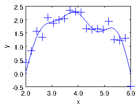
Figure 1.8: The result of the fit of sinusoids up to M=5 to a noisy
dataset of size N=20. The points are the input data. The curve is
constructed by using the
yfit expression on an
xfit array of some convenient length spanning the x-range, and
then simply plotting
yfit versus
xfit.
Exercise 1. Data fitting
1. Given a set of N values yi of a function y(x) at the positions
xi, write a short code to fit a polynomial having order one less
than N (so there are N coefficients of the polynomial) to the data.
Obtain a set of (N=) 6 numbers from
http://silas.psfc.mit.edu/22.15/15numbers.html
(or if that is not accessible use yi=[0.892,1.44,1.31,1.66,1.10,1.19]).
Take the values yi to be at the positions
xi=[0.0,0.2,0.4,0.6,0.8,1.0]. Run your code on this data and find the
coefficients cj.
Plot together (on the same plot) the resulting fitted polynomial
representing y(x) (with sufficient resolution to give a smooth
curve) and the original data points, over the domain 0 ≤ x ≤ 1.
Submit the following as your solution:
- Your code in a computer format that is capable of being
executed.
- The numeric values of your coefficients cj, j=1,N.
- Your plot.
- Brief commentary ( < 300 words) on what problems you faced and how you solved them.
2. Save your code from part 1. Make a copy of it with a new name and
change the new code as needed to fit (in the linear least squares sense) a
polynomial of order possibly lower than N−1 to a set of data xi,
yi (for which the points are in no particular order).
Obtain a pair of data sets of length (N=) 20 numbers xi, yi
from the same URL by changing the entry in the "Number of Numbers"
box. (Or if that is inaccessible, generate your own data set from random
numbers added to a line.) Run your code on that data to produce the fitting
coefficients cj when the number of coefficients of the polynomial
is (M=) (a) 1, (b) 2, (c) 3. That is: constant, linear, quadratic.
Plot the fitted curves
and the original data points on the same plot(s) for all three cases.
Submit the following as your solution:
- Your code in a computer format that is capable of being
executed.
- Your coefficients cj, j=1,M, for three cases (a), (b), (c).
- Your plot(s).
- Very brief remarks on the extent to which the coefficients are
the same for the three cases.
- Can your code from this part also solve the problem of part 1?