| HEAD | PREVIOUS |
|
dy
|
|
dNy
|
| (2.1) |
| (2.2) |
| (2.3) |
| (2.4) |
| (2.5) |
| (2.6) |
| B=B |
^
z
|
| (2.7) |
| (2.8) |
| (2.9) |
| (2.10) |
|
df
|
| (2.11) |
| (2.12) |
| (2.13) |
| (2.14) |
| (2.15) |
|
|
∆
|
| (2.17) |
| (2.18) |
| (2.19) |
| (2.20) |
| (2.21) |
| (2.22) |
| (2.23) |
| (2.24) |
| (2.25) |
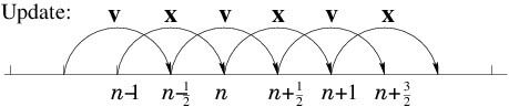 One trap for the unwary in a Leap-Frog scheme is the specification of
initial values. If we want to
calculate an orbit which has specified initial position x0
and velocity v0 at time t=t0, then it is not sufficient
simply to put the velocity initially equal to the specified
v0. That is because the first velocity, which governs the
position step from t0 to t1 is not v0, but
v1/2. To start the integration off correctly, therefore, we
must take a half-step in velocity by putting v1/2 = v0+ a0 (t1−t0)/2, before beginning the standard
integration.
Leap-Frog schemes generally possess important conservation properties
such as conservation of momentum, that
can be essential for realistic simulation with a large number of
particles.
One trap for the unwary in a Leap-Frog scheme is the specification of
initial values. If we want to
calculate an orbit which has specified initial position x0
and velocity v0 at time t=t0, then it is not sufficient
simply to put the velocity initially equal to the specified
v0. That is because the first velocity, which governs the
position step from t0 to t1 is not v0, but
v1/2. To start the integration off correctly, therefore, we
must take a half-step in velocity by putting v1/2 = v0+ a0 (t1−t0)/2, before beginning the standard
integration.
Leap-Frog schemes generally possess important conservation properties
such as conservation of momentum, that
can be essential for realistic simulation with a large number of
particles.
| (2.26) |
| (2.27) |
|
d
| z=Az |
|
d
| z=λz |
| (2.28) |
| (2.29) |
| (2.30) |
|
d2y
| = −1 |
| A y + B |
dy
| + C |
d2y
| + D |
d3y
| = E |
|
d2 y
| = 2 | ⎛ ⎝ |
dy
| ⎞ ⎠ |
2 | − y3 |
| (2.31) |
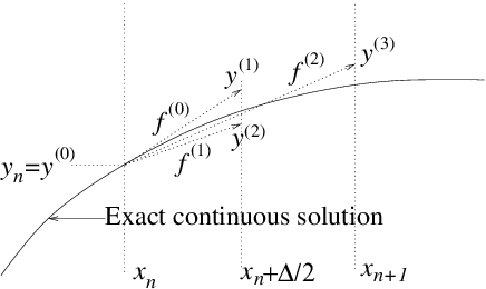
| (a) | Integrate
term by term to find the solution for y to third-order in x. | |||
| (b) | Suppose y1 = f0 x. Find y1−y(x) to second-order in x. | |||
| (c) | Now consider y2 = f(y1,x) x, show that it is equal to f(y,x)x plus a term that is third-order in x. | |||
| (d) | Hence find y2−y to second-order in x. | |||
| (e) | Finally show that y3 = 1/2 ( y1+ y2) is equal to y accurate to second-order in x. |
|
|
|
| HEAD | NEXT |