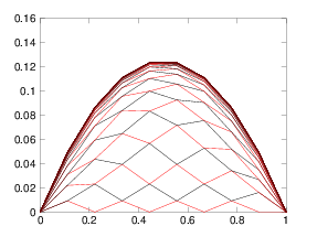
Figure 6.1: (a) One dimensional Gauss Seidel odd-even iteration produces
successive solutions for each half-step that form a web that
progresses upwards toward the solution. (b) In two dimensions the
alternate squares to be updated are all the red (lighter shaded), then all the black.
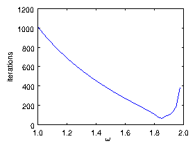
Figure 6.2: Number of iterations required to converge a SOR solution of
Poisson's equation with uniform source on a mesh of length
N
j=32. It is declared converged when the maximum ψ-change
in a step is less than 10
−6 ψ
max. The minimum
number of iterations is found to be 63 at ω = 1.85. This
should be compared with theoretical values of
ln(10
6)(N
j/2π)=70 at
ω = 2/(1+π/N
j)=1.821.
 (a)
(a)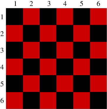 (b)
(b)