Chapter 3
Collisions in Plasmas
3.1 Binary collisions between charged particles
Reduced-mass for binary collisions:
Two particles interacting with each other have forces
F12 force on 1 from 2.
F21 force on 2 from 1.
By Newton's 3rd law, F12 = − F21.
Equations of motion:
|
m1 |
⋅⋅
r
|
1
|
= F12 ; m2 |
⋅⋅
r
|
2
|
= F21 |
| (3.1) |
Combine to get
|
|
⋅⋅
r
|
1
|
− |
⋅⋅
r
|
2
|
= F12 | ⎛
⎝
|
1
m1
|
+ |
1
m2
| ⎞
⎠
|
|
| (3.2) |
which may be written
|
|
m1m2
m1 + m2
|
|
d2
dt2
|
(r1 − r2 ) = F12 |
| (3.3) |
If F12 depends only on the difference vector r1 − r2,
then this equation is identical to the equation of a particle
of "Reduced Mass" mr ≡ [(m1m2)/(m1 + m2 )]
moving at position r ≡ r1 − r2 with respect
to a fixed center of force:
This is the equation we analyse, but actually particle
2 does move. And we need to recognize that when
interpreting mathematics.
If F21 and r1 − r2 are always parallel, then a
general form of the trajectory can be written as an integral.
To save time we specialize immediately to the Coulomb force
Figure 3.1: Geometry of the collision orbit
Solution of this standard (Newton's) problem:
Angular momentum is conserved:
|
mr r2 |
⋅
θ
|
= const. = mr bv1 (θ clockwise from symmetry) |
| (3.6) |
Substitute u ≡ 1/r then · θ = [(bv1)/(r2)] = u2 bv1
Also
| |
|
|
|
d
dt
|
|
1
u
|
= − |
1
u2
|
|
du
dθ
|
|
⋅
θ
|
= − bv1 |
du
dθ
|
|
| | (3.7) |
| |
|
| − bv1 |
d2u
dθ2
|
|
⋅
θ
|
= − ( bv1)2 u2 |
d2 u
dθ2
|
|
| | (3.8) |
|
Then radial acceleration is
|
|
⋅⋅
r
|
− r |
⋅
θ
|
2
|
= − (bv1)2 u2 | ⎛
⎝
|
d2 u
dθ2
|
+ u | ⎞
⎠
|
= |
F12
mr
|
|
| (3.9) |
i.e.
|
|
d2 u
dθ2
|
+ u = − |
q1 q2
4 πϵ0
|
|
1
mr ( bv1 )2
|
|
| (3.10) |
This orbit equation has the elementary solution
|
u ≡ |
1
r
|
= C cosθ − |
q1 q2
4 πϵ0
|
|
1
mr ( bv1 )2
|
|
| (3.11) |
The sinθ term is absent by symmetry.
The other constant of integration, C, must be determined
by initial condition. At initial (far distant) angle,
θ1, u1 = [1/(∞)] = 0 .
So
|
0 = C cosθ1 − |
q1 q2
4 πϵ0
|
|
1
mr ( bv1 )2
|
|
| (3.12) |
There:
|
|
⋅
r
|
1
|
= − v1 = − bv1 |
du
dθ
|
|1 = + bv1 C sinθ1 |
| (3.13) |
Hence
|
tanθ1 = |
sinθ1
cosθ1
|
= |
−1 / Cb
q1 q2
4 πϵ0
|
|
1
mr ( bv1 )2
|
/ C |
|
= − |
b
b90
|
|
| (3.14) |
where
|
b90 ≡ |
q1 q2
4 πϵ0
|
|
1
mr v12
|
. |
| (3.15) |
Notice that tanθ1 = −1 when b = b90. This
is when θ1 = −45° and χ = 90°. So
particle emerges at 90° to initial direction when
|
b = b90 "90° impact parameter" |
| (3.16) |
Finally:
|
C = − |
1
b
|
cosecθ1 = − |
1
b
|
| ⎛
⎝
|
1 + |
b902
b2
| ⎞
⎠
|
1/2
|
|
| (3.17) |
3.1.1 Frames of Reference
Key quantity we want is the scattering angle but we need
to be careful about reference frames.
Most "natural" frame of ref is "Center-of-Mass" frame,
in which C of M is stationary. C of M has position:
and velocity (in lab frame)
Now
So motion of either particle in C of M frame is a factor times
difference vector, r.
Velocity in lab frame is obtained by adding V to the C of M
velocity, e.g. [(m2 · r)/(m1 + m2)] + V.
Angles of position vectors and velocity differences
are same in all frames.
Angles (i.e. directions) of velocities are not same.
3.1.2 Scattering Angle
In C of M frame is just the final angle of r.
(θ1 is negative)
Figure 3.2: Relation between θ1 and χ.
|
χ = π+ 2 θ1 ; θ1 = |
χ− π
2
|
. |
| (3.23) |
|
tanθ1 = tan | ⎛
⎝
|
χ
2
|
− |
π
2
| ⎞
⎠
|
= − cot |
χ
2
|
|
| (3.24) |
So
But scattering angle (defined as exit velocity angle
relative to initial velocity) in lab frame is different.
Figure 3.3: Collisions viewed in Center of Mass
and Laboratory frame.
Final velocity in CM frame
| |
|
| v1CM ( cosχc, sinχc ) = |
m2
m1 + m2
|
v1 ( cosχc, sinχc ) |
| | (3.27) |
|
[ χc ≡ χ and v1 is initial relative velocity].
Final velocity in Lab frame
|
v′L = v′CM + V= | ⎛
⎝
|
V + |
m2v1
m1 + m2
|
cosχc , |
m2v1
m1 + m2
|
sinχc | ⎞
⎠
|
|
| (3.28) |
So angle is given by
|
cotχL = |
|
= |
V
v1
|
|
m1 + m2
m2
|
cosecχc + cotχc |
| (3.29) |
For the specific case when m2 is initially a
stationary target in lab frame, then
This is exact.
Small angle approximation (cotχ→ [ 1/(χ)]) , cosecχ→ [ 1/(χ)] gives
|
|
1
χL
|
= |
m1
m2
|
|
1
χc
|
+ |
1
χc
|
⇔ χL = |
m2
m1 + m2
|
χc |
| (3.32) |
So small angles are proportional, with ratio set by the
mass-ratio of particles.
3.2 Differential Cross-Section for Scattering by
Angle
By definition the cross-section, σ, for any
specified collision process when a particle is passing
through a density n2 of targets is such that the
number of such collisions per unit path length is
n2σ.
Sometimes a continuum of types of collision is considered,
e.g. we consider collisions at different angles (χ)
to be distinct. In that case we usually discuss
differential cross-sections (e.g [(dσ)/(dχ)])
defined such that number of collisions in an (angle)
element dχ per unit path length is n2 [(dσ)/(dχ)] dχ.
[Note that [(dσ)/(dχ)] is just notation for a number.
Some authors just write σ(χ), but I find that less
clear.]
Normally, for scattering-angle discrimination we discuss the
differential cross-section per unit solid angle:
This is related to scattering angle integrated over all
azimuthal directions of scattering by:
Figure 3.4: Scattering angle and solid angle relationship.
So that since
we have
Now, since χ is a function (only) of the impact
parameter, b, we just have to determine the number of
collisions per unit length at impact parameter b.
Figure 3.5: Annular volume corresponding to db.
Think of the projectile as dragging along an annulus
of radius b and thickness db for an elementary
distance along its path, dl. It thereby drags through
a volume:
Therefore in this distance it has encountered a total
number of targets
at impact parameter b(db). By definition this is equal to
dl[(dσ)/db] db n2. Hence the
differential cross-section for scattering (encounter) at
impact parameter b is
Again by definition, since χ is a function of b
|
|
dσ
dχ
|
dχ = |
dσ
db
|
db ⇒ |
dσ
dχ
|
= |
dσ
db
|
| ⎢
⎢
|
db
dχ
| ⎢
⎢
|
. |
| (3.40) |
[db/dχ is negative but differential cross-sections are
positive.]
Substitute and we get
|
|
dσ
dΩs
|
= |
1
2 πsinχ
|
|
dσ
db
|
| ⎢
⎢
|
db
dχ
| ⎢
⎢
|
= |
b
sinχ
|
| ⎢
⎢
|
db
dχ
| ⎢
⎢
|
. |
| (3.41) |
[This is a general result for classical collisions.]
For Coulomb collisions, in C of M frame,
|
⇒ |
db
dχ
|
= b90 |
d
dχ
|
cot |
χ
2
|
= − |
b90
2
|
cosec2 |
χ
2
|
. |
| (3.43) |
Hence
This is the Rutherford Cross-Section.
for scattering by Coulomb forces through an angle χ measured
in C of M frame.
Notice that [(dσ)/(dΩs)] → ∞
as χ→ 0.
This is because of the long-range nature of the Coulomb force.
Distant collisions tend to dominate. (χ→ 0⇔b → ∞).
3.3 Relaxation Processes
There are 2 (main) different types of collisional relaxation
process we need to discuss for a test particle moving through
a background of scatterers:
- Energy Loss (or equilibrium)
- Momentum Loss (or angular scattering)
The distinction may be illustrated by a large angle (90°)
scatter
from a heavy (stationary) target.
If the target is fixed, no energy is transferred to it.
So the energy loss is zero (or small if scatterer is
just `heavy'). However, the momentum in the x direction
is completely `lost' in this 90° scatter.
This shows that the timescales for Energy loss and momentum
loss may be very different.
3.3.1 Energy Loss
For an initially stationary target, the final velocity
in lab frame of the projectile is
|
vL′ = | ⎛
⎝
|
m1v1
m1 + m2
|
+ |
m2v1
m1 + m2
|
cosχc , |
m2v1
m1 + m2
|
sinχc | ⎞
⎠
|
|
| (3.48) |
So the final kinetic energy is
| |
|
|
|
1
2
|
m1vL′2 = |
1
2
|
m1v12 | ⎧
⎨
⎩
|
| ⎛
⎝
|
m1
m1 + m2
| ⎞
⎠
|
2
|
+ |
2 m1m2
( m1+m2 )2
|
cosχc |
| | (3.49) |
| |
|
|
+ |
m22
( m1 + m2 )2
|
( cos2 χc + sin2 χc ) | ⎫
⎬
⎭
|
|
| | (3.50) |
| |
|
|
|
1
2
|
m1v12 | ⎧
⎨
⎩
|
1 + |
2m1m2
( m1+m2 )2
|
( cosχc − 1) | ⎫
⎬
⎭
|
|
| | (3.51) |
| |
|
|
1
2
|
m1v12 | ⎧
⎨
⎩
|
1 − |
2m1m2
( m1+m2 )2
|
2 sin2 |
χc
2
| ⎫
⎬
⎭
|
|
| | (3.52) |
|
Hence the kinetic energy lost is ∆K = K − K′
| |
|
|
|
1
2
|
m1v12 |
4 m1m2
( m1+m2 )2
|
sin2 |
χc
2
|
|
| | (3.53) |
| |
|
|
1
2
|
m1v12 |
4m1m2
( m1+m2 )2
|
|
1
|
[using cot |
χc
2
|
= |
b
b90
|
] |
| | (3.54) |
|
(exact).
For small angles χ << 1 i.e. b / b90 >> 1 this
energy lost in a single collision is approximately
|
| ⎛
⎝
|
1
2
|
m1v12 | ⎞
⎠
|
|
4 m1m2
( m1+m2 )2
|
| ⎛
⎝
|
b90
b
| ⎞
⎠
|
2
|
|
| (3.55) |
If what we are asking is: how fast does the projectile lose
energy? Then we need add up the effects of all
collisions in an elemental length dl at all relevant
impact parameters.
The contribution from impact parameter range db at b will equal
the number of targets encountered times ∆K:
|
|
n2dl2 πb d b
encounters
|
|
|
|
1
2
|
m1v12 |
4m1m2
( m1+m2 )2
|
| ⎛
⎝
|
b90
b
| ⎞
⎠
|
2
|
Loss per encounter (∆K)
|
|
| (3.56) |
This must be integrated over all b to get total energy loss.
|
dK = n2 dlK |
4 m1m2
( m1+m2 )2
|
| ⌠
⌡
|
| ⎛
⎝
|
b90
b
| ⎞
⎠
|
2
|
2 πb d b |
| (3.57) |
so
|
|
dK
dl
|
= K n2 |
m1 m2
( m1 + m2 )2
|
8 πb902 [ ln| b | ]maxmin |
| (3.58) |
We see there is a problem both limits of the integral
(b → 0, b → ∞) diverge logarithmically.
That is because the formulas we are integrating are approximate.
- We are using small-angle approx for ∆K.
- We are assuming the Coulomb force applies but this is a
plasma so there is screening.
3.3.2 Cut-offs Estimates
1. Small-angle approx breaks down around b = b90. Just truncate
the integral there; ignore contributions from b < b90. Actually
this apparently arbitrary approximation is rigorously justified by an
integration of the exact (not small angle) loss expression.
|
| ⌠
⌡
|
|
2bdb
(b/b90)2+1
|
= b902ln[(b/b90)2+1] →b2→ 0 as b→0. |
|
So if we had not made the small-angle approximation (which is here not
mathematically essential) we would not have had a small-b
divergence, we would have got zero from the lower limit.
2. Large-b cut-off arises because the Coulomb potential does not apply to
arbitrarily large distances. Debye Shielding says really the potential varies as
so approximate this by cutting off integral at b = λD
equivalent to
So the cut-offs can be taken as bmin = b90 and bmax = λD .
| |
|
|
K n2 |
m1m2
(m1+m2 )2
|
8 πb902 ln| Λ | |
| | (3.60) |
| |
|
|
λD
b90
|
= | ⎛
⎝
|
ϵ0 Te
n e2
| ⎞
⎠
|
1/2
|
| / |
| ⎛
⎝
|
q1q2
4 πϵ0 mrv12
| ⎞
⎠
|
|
| | (3.61) |
|
So Coulomb Logarithm is `lnΛ'
|
Λ = |
λD
b90
|
= | ⎛
⎝
|
ϵ0 Te
n e2
| ⎞
⎠
|
1/2
|
| / |
| ⎛
⎝
|
q1q2
4 πϵ0 mrv12
| ⎞
⎠
|
|
| (3.62) |
Because these cut-offs are in ln term result is not
sensitive to their exact values.
One commonly uses Collision Frequency. Energy Loss
Collision Frequency is
|
νK ≡ v1 |
1
K
|
|
dK
dl
|
= n2 v1 |
m1m2
( m1 + m2 )2
|
8 πb902 ln| Λ | |
| (3.63) |
Substitute for b90 and mr (in b90)
| |
|
|
n2 v1 |
m1m2
( m1+m2 )2
|
8 π | ⎡
⎢
⎣
|
q1q2
| ⎤
⎥
⎦
|
2
|
lnΛ |
| | (3.64) |
| |
|
| n2 |
q12q22
( 4 πϵ0 )2
|
|
8 π
m1m2v13
|
lnΛ |
| | (3.65) |
|
Collision time τK ≡ 1/νK
Effective (Energy Loss) Cross-section
[ 1/K [dK/(d l)] = σKn2 ]
|
σK = νK / n2v1 = |
q12q22
( 4 πϵ0 )2
|
|
8 π
m1m2v14
|
lnΛ. |
| (3.66) |
3.3.3 Momentum Loss
Loss of x-momentum in 1 collision is
| |
|
| | (3.67) |
| |
|
|
m1v1 | ⎧
⎨
⎩
|
1 − | ⎛
⎝
|
m1
m1+m2
|
+ |
m2
m1+m2
|
cosχc | ⎞
⎠
| ⎫
⎬
⎭
|
|
| | (3.68) |
| |
|
|
px |
m2
m1+m2
|
( 1 − cosχc ) |
| | (3.69) |
| |
|
| px |
m2
m1+m2
|
|
χc2
2
|
= px |
m2
m1+m2
|
|
2 b902
b2
|
|
| | (3.70) |
|
(small angle approx).
Hence rate of momentum loss can be obtained using an integral
identical to the energy loss but with the above parameters:
| |
|
|
n2p | ⌠
⌡
|
bmax
bmin
|
|
m2
m1 + m2
|
|
2 b902
b2
|
2 πb d b |
| | (3.71) |
| |
|
| n2 p |
m2
m1 + m2
|
4π b902 lnΛ |
| | (3.72) |
|
Note for future reference:
|
|
dp
dt
|
= v1 |
dp
dl
|
= n2v12 |
m1m2
m1 + m2
|
4 πb902 lnΛ . |
| (3.73) |
Therefore Momentum Loss.
Collision Frequency
| |
|
|
v1 |
1
p
|
|
dp
dl
|
= n2v1 |
m2
m1+m2
|
4 πb902 lnΛ |
| | (3.74) |
| |
|
|
n2v1 |
m2
m1+m2
|
4 π | ⎡
⎢
⎣
|
q1q2
| ⎤
⎥
⎦
|
2
|
lnΛ |
| | (3.75) |
| |
|
| n2 |
q12q22
( 4 πϵ0 )2
|
|
4 π(m1+m2)
m2m12v13
|
lnΛ |
| | (3.76) |
|
Collision Time τp = 1/νp
Cross-Section (effective) σ = νp/n2v1
Notice ratio
|
|
Energy Loss νK
Momentum loss νp
|
= |
2
m1m2
|
| / |
|
m1+m2
m2m12
|
= |
2 m1
m1 + m2
|
|
| (3.77) |
This is
Third case, e.g. electrons → ions shows that mostly
the angle of velocity scatters. Therefore Momentum
`Scattering' time is often called `90° scattering'
time to `diffuse' through 90° in angle.
3.3.4 `Random Walk' in angle
When m1 << m2, energy loss << momentum loss.
Hence |vL′| ≅ v1. All that matters is
the scattering angle: χL ≅ χc ≅ 2 b90/b.
Mean angle of total deviation ∆α in length L is zero because all
directions are equally likely.
But:
Mean square angle is
| |
|
|
n2 L | ⌠
⌡
|
bmax
bmin
|
χ2 2 πb d b |
| | (3.81) |
| |
|
| | (3.82) |
|
Spread is `all round' when ―∆α2 ≅ 1.
This is roughly when a particle has scattered 90° on
average. It requires
So can think of a kind of `cross-section' `σ90' for
90° scattering as such that
| |
|
|
1 when L n2 8 π b902 lnΛ = 1 |
| | (3.84) |
| |
|
| | (3.85) |
|
This is 8 lnΛ larger than cross-section for 90°
scattering in single collision.
Be Careful! `σ90' is not a usual type of
cross-section because the whole process is really diffusive in
angle.
Actually all collision processes due to coulomb force are best
treated (in a Mathematical way) as a diffusion in velocity space
→ Fokker-Planck equation.
3.3.5 Summary of different types of collision
The Energy Loss collision frequency is to do with slowing
down to rest and exchanging energy. It is required for
calculating
Equilibration Times (of Temperatures)
Energy Transfer between species.
The Momentum Loss frequency is to do with loss of
directed velocity. It is required for calculating
Mobility: Conductivity/Resistivity
Viscosity
Particle Diffusion
Energy (Thermal) Diffusion
Usually we distinguish between electrons and ions because
of their very different mass:
Energy Loss [Stationary Targets]
Momentum Loss
| |
|
|
ne |
e4
( 4 πϵ0 )2
|
|
8 π
me2 ve3
|
lnΛ pνee = Kνee × | ⎡
⎣
|
me+me
2me
|
= 1 | ⎤
⎦
|
|
| |
| |
|
|
ni |
Z2e4
( 4 πϵ0 )2
|
|
8 π
memive3
|
lnΛ pνei = Kνei × | ⎡
⎣
|
me+mi
2me
|
≅ |
mi
2me
| ⎤
⎦
|
|
| |
| |
|
|
ni |
Z2e4
( 4 πeo )2
|
|
8 π
mi2vi3
|
lnΛ pνii = Kνii × | ⎡
⎣
|
mi+mi
2mi
|
= 1 | ⎤
⎦
|
|
| | (3.86) |
| |
|
| ne |
Ze2e4
( 4 πϵ0 )2
|
|
8 π
mimevi3
|
lnΛ pνie = Kνie × | ⎡
⎣
|
me+mi
2mi
|
≅ |
1
2
| ⎤
⎦
|
|
| |
|
Sometimes one distinguishes between `transverse diffusion' of
velocity and `momentum loss'. The ratio of these two is
| |
|
|
|
d χL2
d l
|
| / |
| ⎢
⎢
|
1
p
|
|
dp
dl
| ⎢
⎢
|
|
| | (3.87) |
| |
|
| | (3.88) |
|
So
Hence
| |
|
| | (3.92) |
| |
|
|
2 pνei = Kνee |
ni
ne
|
Z2 ( = Zνee ) ( = `νei′) |
| | (3.93) |
| |
|
|
pνii = Kνii ( = νii!! ) (Like Ions) |
| | (3.94) |
| |
|
|
2me
mi
|
pνie = |
me
mi
|
Kνie = Kνii = νii |
| | (3.95) |
|
[But note: ions are slowed down by electrons long before being
angle scattered.]
3.4 Thermal Distribution Collisions
So far we have calculated collision frequencies with stationary
targets and single-velocity projectiles but generally we shall
care about thermal (Maxwellian) distributions (or nearly
thermal) of both species. This is harder to calculate and
we shall resort to some heuristic calculations.
3.4.1 e → i
Very rare for thermal ion velocity to be ∼ electron.
So ignore ion motion.
Average over electron distribution.
Momentum loss to ions from (assumed) drifting
Maxwellian electron distribution:
|
fe (v) = ne | ⎛
⎝
|
me
2 πTe
| ⎞
⎠
|
3/2
|
exp | ⎡
⎣
|
− |
m( v− vd )2
2T
| ⎤
⎦
|
|
| (3.96) |
Each electron in this distribution is losing momentum to the ions
at a rate given by the collision frequency
|
νp = ni |
qe2qi2
( 4 πϵ0 )2
|
|
4 π( me+mi )
mime2v3
|
lnΛ |
| (3.97) |
so total rate of loss of momentum is given by (per unit volume)
|
− |
dp
dt
|
= | ⌠
⌡
|
fe(v) νp(v) mev d3v
|
| (3.98) |
To evaluate this integral approximately we adopt the following
simplifications.
- Ignore variations of lnΛ with v and just
replace a typical thermal value in Λ = λD/b90(v1).
- Suppose that drift velocity vd is small relative
to the typical thermal velocity, written
ve ≡ √{Te/me} and express fe in terms of
u ≡ [(v)/(ve)] to first order in
ud ≡ [(vd)/(ve)]:
| |
|
|
ne |
1
( 2 π)3/2 ve3
|
exp | ⎡
⎣
|
−1
2
|
( u − ud )2 | ⎤
⎦
|
|
| | (3.99) |
| |
|
|
ne
( 2π)3/2 ve3
|
( 1 + u . ud ) exp | ⎡
⎣
|
−u2
2
| ⎤
⎦
|
= ( 1 + ux ud ) fo |
| | (3.100) |
|
taking x-axis along ud and denoting by fo the
unshifted Maxwellian.
Then momentum loss rate per unit volume
| |
|
| |
| |
|
|
νp (ve) me | ⌠
⌡
|
(1 + ux ud) fo |
ve3
v3
|
vx d3 v |
| | (3.101) |
| |
|
| νp (ve) mevd | ⌠
⌡
|
|
ux2
u3
|
fo d3 v |
| |
|
To evaluate this integral, use the spherical symmetry
of fo to see that:
| |
|
|
|
1
3
|
| ⌠
⌡
|
|
ux2 + uy2 + uz2
u3
|
fo d3 v= |
1
3
|
| ⌠
⌡
|
|
u2
u3
|
fo d3 v |
| |
| |
|
|
|
1
3
|
| ⌠
⌡
|
α
0
|
|
ve
v
|
fo 4 πv2 d v |
| |
| |
|
|
|
2 π
3
|
ve | ⌠
⌡
|
α
0
|
fo 2 v d v |
| |
| |
|
|
|
2 π
3
|
ve |
ne
( 2 π)3/2 ve3
|
| ⌠
⌡
|
α
0
|
exp | ⎛
⎝
|
−v2
2ve2
| ⎞
⎠
|
dv2 |
| |
| |
|
|
2 π
3
|
|
ne
( 2 π)3/2
|
2 = |
2
3 ( 2 π)1/2
|
ne . |
| | (3.102) |
|
Thus the Maxwell-averaged momentum-loss frequency is
|
− |
1
p
|
|
dp
dt
|
≡ |
ν
|
ei
|
= |
2
3 ( 2 π)1/2
|
νp (ve) |
| (3.103) |
(where p = mevdne is the momentum per unit volume
attributable to drift).
| |
|
|
|
2
3 ( 2 π)1/2
|
ni |
qe2qi2
( 4 πϵ0 )2
|
|
4 π( me+mi )
mi me2 ve3
|
lnΛe |
| | (3.104) |
| |
|
|
2
3 ( 2 π)1/2
|
ni | ⎛
⎝
|
Ze2
4 πϵ0
| ⎞
⎠
|
2
|
|
4 π
me1/2 Te3/2
|
lnΛe |
| | (3.105) |
|
(substituting for thermal electron velocity, ve,
and dropping [(me)/(mi)] order term), where
Ze = qi.
This is the standard form of electron collision frequency.
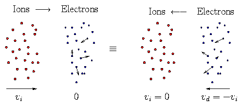
3.4.2 i → e
Ion momentum loss to electrons can be treated by a
simple Galilean transformation of the e → i
case because it is still the electron thermal motions
that matter.
Figure 3.6: Ion-electron collisions are
equivalent to electron-ion collisions in a moving reference frame.
Rate of momentum transfer, [dp/dt], is same in both
cases:
Hence |pe|νei = |pi| νie or
|
|
ν
|
ie
|
= |
|pe|
|pi|
|
|
ν
|
ei
|
= |
neme
nimi
|
|
ν
|
ei
|
|
| (3.107) |
(since drift velocities are the same).
Ion momentum loss to electrons has much lower collision
frequency than e → i because ions possess
so much more momentum for the same velocity.
3.4.3 i → i
Ion-ion collisions can be treated somewhat like e → i
collisions except that we have to account for moving targets
i.e. their thermal motion.
Consider two different ion species moving relative to each other
with drift velocity vd; the targets' thermal motion
affects the momentum transfer cross-section.
Using our previous expression for momentum transfer, we can
write the average rate of transfer per unit volume as:
[see 3.73 "note for future reference"]
|
− |
dp
dt
|
= | ⌠
⌡
|
| ⌠
⌡
|
vr |
m1m2
m1+m2
|
vr 4 π b902 lnΛ f1f2 d3 v1 d3 v2 |
| (3.108) |
where vr is the relative velocity (v1−v2) and
b90 is expressed
and mr is the reduced mass
[(m1m2)/(m1+m2)].
Since everything in the integral apart from f1f2 depends only on
the relative velocity, we proceed by transforming the velocity
coordinates from v1,v2 to being expressed in terms of relative
(vr) and average (i.e. individual center of mass velocity, V)
|
vr ≡ v1 − v2 ; V ≡ |
m1v1 + m2v2
m1+m2
|
. |
| (3.110) |
Take f1 and f2 to be shifted Maxwellians in the overall
C of M frame:
|
fj = nj | ⎛
⎝
|
mj
2 πT
| ⎞
⎠
|
3/2
|
exp | ⎡
⎣
|
− |
mj ( vj − vdj )2
2 T
| ⎤
⎦
|
(j = 1, 2) |
| (3.111) |
where m1vd1 + m2vd2 = 0. Then
| |
|
|
n1n2 | ⎛
⎝
|
m1
2πT
| ⎞
⎠
|
3/2
|
| ⎛
⎝
|
m2
2 πT
| ⎞
⎠
|
3/2
|
exp | ⎡
⎣
|
− |
m1v12
2 T
|
− |
m2v22
2T
| ⎤
⎦
|
|
| |
| |
|
| × | ⎧
⎨
⎩
|
1 + |
v1 . m1vd1
T
|
+ |
v2 . m2vd2
T
| ⎫
⎬
⎭
|
|
| | (3.112) |
|
to first order in vd. Convert to local CM v-coordinates and
find (after algebra)
| |
|
|
n1n2 | ⎛
⎝
|
M
2πT
| ⎞
⎠
|
3/2
|
| ⎛
⎝
|
mr
2πT
| ⎞
⎠
|
3/2
|
exp | ⎡
⎣
|
− |
MV2
2T
|
− |
mrvr2
2T
| ⎤
⎦
|
|
| |
| |
|
| × | ⎧
⎨
⎩
|
1 + |
mr
T
|
vd . vr | ⎫
⎬
⎭
|
|
| | (3.113) |
|
where M = m1+m2. Note also that (it can be shown) that the
Jacobian of the transformation is unity
d3v1 d3v2 = d3vrd3V.
Hence
| |
|
|
| ⌠
⌡
|
| ⌠
⌡
|
vr mr vr 4 π b902lnΛ n1n2 | ⎛
⎝
|
M
2πT
| ⎞
⎠
|
3/2
|
| ⎛
⎝
|
mr
2πT
| ⎞
⎠
|
3/2
|
|
| |
| |
|
| exp | ⎛
⎝
|
− |
MV2
2T
| ⎞
⎠
|
exp | ⎛
⎝
|
− |
mrvr2
2T
| ⎞
⎠
|
| ⎧
⎨
⎩
|
1 + |
mr
T
|
vd . vr | ⎫
⎬
⎭
|
d3 vr d3 V |
| | (3.114) |
|
and since nothing except the exponential depends on V, that
integral can be done:
|
− |
dp
dt
|
= | ⌠
⌡
|
vr mrvr4πb902 lnΛ n1n2 | ⎛
⎝
|
mr
2πT
| ⎞
⎠
|
3/2
|
exp | ⎛
⎝
|
−mrvr2
2π
| ⎞
⎠
|
| ⎧
⎨
⎩
|
1 + |
mr
T
|
vd . vr | ⎫
⎬
⎭
|
d3 vr |
| (3.115) |
This integral is of just the same type as for e−i collisions,
i.e.
| |
|
|
vd vri mr 4 π b902 (vri) lnΛt n1n2 | ⌠
⌡
|
|
ux2
u3
|
|
^
f
|
o
|
(vr) d3 vr |
| |
| |
|
| vdvri mr 4 π b902 (vri) ln Λt n1n2 |
2
3 ( 2π)1/2
|
|
| | (3.116) |
|
where vri ≡ √{[T/(mr)]}, b902 (vri) is
the ninety degree impact parameter evaluated at velocity vtr,
and ∧fo is the
normalized Maxwellian.
|
− |
dp
dt
|
= |
2
3 ( 2π)1/2
|
| ⎛
⎝
|
q1q2
4 πϵ0
| ⎞
⎠
|
2
|
|
4 π
mr2vri3
|
lnΛt n1n2 mr vd |
| (3.117) |
This is the general result for momentum exchange rate
between two Maxwellians drifting at small relative
velocity vd.
To get a collision frequency is a matter of deciding which
species is stationary and so what the momentum density of
the moving species is. Suppose we regard 2 as targets then
momentum density is n1m1vd so
|
|
ν
|
12
|
= |
1
n1m1vd
|
|
dp
dt
|
= |
2
3 ( 2 π)1/2
|
n2 | ⎛
⎝
|
q1q2
4 πϵ0
| ⎞
⎠
|
2
|
|
4 π
mr vri3
|
|
lnΛt
m1
|
. |
| (3.118) |
This expression works immediately for electron-ion collisions
substituting mr ≅ me, recovering previous.
For equal-mass ions mr = [(mi2)/(mi+mi)] = 1/2 mi and
vri = √{[T/(mr)]} = √{[2T/(mi)]}.
Substituting, we get
|
|
ν
|
ii
|
= |
1
3 π1/2
|
ni | ⎛
⎝
|
q1q2
4 πϵ0
| ⎞
⎠
|
2
|
|
4 π
mi1/2 Ti3/2
|
lnΛ |
| (3.119) |
that is, [ 1/(√2 )] times the e−i
expression but with ion parameters substituted.
[Note, however, that we have considered the ion
species to be different.]
3.4.4 e → e
Electron-electron collisions are covered by the same formalism,
so
|
|
ν
|
ee
|
= |
1
3 π1/2
|
ne | ⎛
⎝
|
e2
4 πϵ0
| ⎞
⎠
|
2
|
|
4 π
me1/2 Te3/2
|
lnΛ . |
| (3.120) |
However, the physical case under discussion is not so
obvious; since electrons are indistiguishable how do we
define two different "drifting maxwellian"
electron populations? A more specific discussion
would be needed to make this rigorous.
Generally νee ∼ νei/ √2 :
electron-electron collision frequency ∼ electron-ion
(for momentum loss).
3.4.5 Summary of Thermal Collision Frequencies
For momentum loss:
| |
|
|
|
√2
|
ni | ⎛
⎝
|
Ze2
4 πϵ0
| ⎞
⎠
|
2
|
|
4 π
me1/2 Te3/2
|
lnΛe . |
| | (3.121) |
| |
|
|
|
1
√2
|
|
ν
|
ei
|
. (electron parameters) |
| | (3.122) |
| |
|
| | (3.123) |
| |
|
|
√2
|
ni′ | ⎛
⎝
|
qiqi′
4 πϵ0
| ⎞
⎠
|
2
|
|
4 π
mi1/2 Ti3/2
|
| ⎛
⎝
|
mi′
mi+mi′
| ⎞
⎠
|
1/2
|
lnΛi |
| | (3.124) |
|
Energy loss Kν related to the above (pν) by
Transverse `diffusion' of momentum ⊥ ν,
related to the above by:
3.5 Applications of Collision Analysis
3.5.1 Energetic (`Runaway') Electrons
Consider an energetic (1/2 me v12 >> T)
electron travelling through a plasma. It is slowed down
(loses momentum) by collisions with electrons and
ions (Z), with collision frequency:
| |
|
|
νee = ne |
e4
( 4 πϵ0)2
|
|
8 π
me2 v13
|
lnΛ |
| | (3.127) |
| |
|
| | (3.128) |
|
Hence (in the absence of other forces)
This is equivalent to saying that the electron experiences an
effective `Frictional' force
| |
|
|
|
d
dt
|
(mev) = − | ⎛
⎝
|
1 + |
Z
2
| ⎞
⎠
|
νee me v |
| | (3.131) |
| |
|
| − | ⎛
⎝
|
1 + |
Z
2
| ⎞
⎠
|
ne |
e4
( 4 πϵ0 )2
|
|
8 π lnΛ
mev2
|
|
| | (3.132) |
|
Notice
- for Z=1 slowing down is 2/3 on
electrons 1/3 ions
- Ff decreases with v increasing.
Suppose now there is an electric field, E. The electron
experiences an accelerating Force.
Total force
|
F = |
d
dt
|
(mv) = −eE + Ff = −eE − | ⎛
⎝
|
1 + |
Z
2
| ⎞
⎠
|
ne |
e4
( 4 πϵ0 )2
|
|
8 πlnΛ
mev2
|
|
| (3.133) |
Two Cases (When E is accelerating)
- | eE | < | Ff |: Electron Slows Down
- | eE | > | Ff |: Electron Speeds Up!
Once the electron energy exceeds a certain value its velocity
increases continuously and the friction force becomes less
and less effective. The electron is then said to have
become a `runaway'.
Condition:
|
|
1
2
|
mev2 > | ⎛
⎝
|
1 + |
Z
2
| ⎞
⎠
|
ne |
e4
( 4 πϵ0 )2
|
|
8 πlnΛ
2 e E
|
|
| (3.134) |
3.5.2 Plasma Resistivity (DC)
Consider a bulk distribution of electrons in an electric field.
They tend to be accelerated by E and decelerated by
collisions.
In this case, considering the electrons as a whole, no loss of
total electron momentum by e−e collisions. Hence the friction
force we need is just that due to ―νei.
If the electrons have a mean drift velocity vd ( << vthe)
then
|
|
d
dt
|
(mevd) = − e E − |
ν
|
ei
|
me vd |
| (3.135) |
Hence in steady state
The current density is then
Now generally, for a conducting medium we define the
conductivity, σ, or resistivity, η, by
|
j = σE ; ηj = E | ⎛
⎝
|
σ = |
1
η
| ⎞
⎠
|
|
| (3.138) |
Therefore, for a plasma,
Substitute the value of ―νei and we get
| |
|
|
|
ni Z2
ne
|
· |
e2 me1/2 8 π lnΛ
|
|
| | (3.140) |
| |
|
|
Z e2 me1/2 8 π lnΛ
|
(for a single ion species). |
| | (3.141) |
|
Notice
- Density cancels out because more electrons means (a) more
carriers but (b) more collisions.
- Main dependence is η ∝ Te−3/2.
High electron temperature implies low resistivity
(high conductivity).
- This expression is only approximate because the current
tends to be carried by the more energetic electrons, which have
smaller νei; thus if we had done a proper average over
f(ve) we expect a lower numerical value. Detailed
calculations give
|
η = 5.2 ×10⁻⁵ |
lnΛ
( Te/eV )3/2
|
Ωm |
| (3.142) |
for Z = 1 (vs. our expression ≅ 10−4).
This is `Spitzer' resistivity. The detailed calculation value is
roughly a factor of two smaller than our calculation, which is not a
negligible correction!
3.5.3 Diffusion
For motion parallel to a magnetic field if we take a
typical electron, with velocity v|| ≅ vte
it will travel a distance approximately
before being pitch-angle scattered enough to have its velocity
randomised. [This is an order-of-magnitude calculation so we
ignore ―νee.] l is the mean free path.
Roughly speaking, any electron does a random walk along the
field with step size l and step frequency ―νei.
Thus the diffusion coefficient of this process is
|
De|| ≅ le2 |
ν
|
ei
|
≅ |
vte2
|
∼ |
T5/2
n
|
. |
| (3.144) |
Similarly for ions
|
Di|| ≅ li2 |
ν
|
ii
|
≅ |
vti2
|
∼ |
T5/2
n
|
|
| (3.145) |
Notice
|
|
ν
|
ii
|
/ |
ν
|
ei
|
≅ | ⎛
⎝
|
me
mi
| ⎞
⎠
|
1/2
|
≅ |
vti
vte
|
(if Te ≅ Ti) |
| (3.146) |
Hence le ≅ li
Mean free paths for electrons and ions are ∼ same.
The diffusion coefficients are in the ratio
|
|
Di
De
|
≅ | ⎛
⎝
|
me
mi
| ⎞
⎠
|
1/2
|
: Ions diffuse slower in parallel direction. |
| (3.147) |
Diffusion Perpendicular to Mag. Field is different
Figure 3.7: Cross-field diffusion by collisions
causing a jump in the gyrocenter (GC) position.
Roughly speaking, if electron direction is changed by
∼ 90° the Guiding Centre moves by a distance
∼ rL. We may think of this as a random walk
with step size ∼ rL and frequency ―νei.
Hence
|
De⊥ ≅ rLe2 |
ν
|
ei
|
≅ |
vte2
Ωe2
|
|
ν
|
ei
|
|
| (3.148) |
Ion transport is similar but both require a discussion of the effects
of like and unlike collisions.
Particle transport occurs only via unlike collisions.
To show this we consider in more detail the change in guiding
center position at a collision.
Recall
m· v = q v∧B
which leads to
|
v⊥ = |
q
m
|
rL ∧B (perp. velocity only). |
| (3.149) |
This gives
At a collision the particle position does not change
(instantaneously) but the guiding center position
(r0) does.
|
r0′+ rL′ = r0 + rL ⇒ ∆r0 ≡ r0′− r0 = − (rL′− rL) |
| (3.151) |
Change in rL is due to the momentum change caused
by the collision:
|
rL′− rL = |
B
q B2
|
∧m(v′⊥ − v⊥) ≡ |
B
q B2
|
∧∆(m v⊥) |
| (3.152) |
So
|
∆ r0 = − |
B
q B2
|
∧∆(m v⊥). |
| (3.153) |
The total momentum conservation means that ∆(mv⊥)
for the two particles colliding is equal and opposite. Hence, from
our equation, for like particles, ∆r0 is equal and
opposite. The mean position of guiding centers of two colliding like
particles (r01 + r02)/2 does not change.
No net cross field particle (guiding center) shift.
Unlike collisions (between particles of different charge q)
do produce net transport of particles of either type. And
indeed may move r01 and r02 in same direction if they have
opposite charge.
|
Di⊥ ≅ rLi2 |
pν
|
ie
|
≅ |
vti2
Ωi2
|
|
pν
|
ie
|
|
| (3.154) |
Notice that
rLi2 / rLe2 ≅ mi/me ; ―pνie /―νei ≅ [(me)/(mi)]
So Di⊥/De⊥ ≅ 1 (for equal temperatures).
Collisional diffusion rates of particles are same for
ions and electrons.
However energy transport is different because it
can occur by like-like collisions.
Thermal Diffusivity:
| |
|
|
rLe2 | ⎛
⎝
|
ν
|
ei
|
+ |
ν
|
ee
| ⎞
⎠
|
∼ rLe2 |
ν
|
ei
|
| ⎛
⎝
|
ν
|
ei
|
∼ |
ν
|
ee
| ⎞
⎠
|
|
| | (3.155) |
| |
|
|
rLi2 | ⎛
⎝
|
pν
|
ie
|
+ |
ν
|
ii
| ⎞
⎠
|
≅ rLi2 |
ν
|
ii
|
| ⎛
⎝
|
ν
|
ii
|
>> |
ν
|
ie
| ⎞
⎠
|
|
| | (3.156) |
| |
|
|
rLi2
rLe2
|
|
|
≅ |
mi
me
|
|
me1/2
mi1/2
|
= | ⎛
⎝
|
mi
me
| ⎞
⎠
|
1/2
|
(equal T) |
| | (3.157) |
|
Collisional Thermal transport by Ions is
greater than by electrons
[factor ∼ (mi/me)1/2 ].
3.5.4 Energy Equilibration
If Te ≠ Ti then there is an exchange of
energy between electrons and ions tending to make
Te = Ti. As we saw earlier
|
Kνei = |
2me
mi
|
pνei = |
me
mi
|
⊥ νei |
| (3.158) |
So applying this to averages.
|
|
Kν
|
ei
|
≅ |
2me
mi
|
|
ν
|
ei
|
( ≅ |
ν
|
ie
|
) |
| (3.159) |
Thermal energy exchange occurs ∼ me/mi
slower than momentum exchange.
(Allows Te ≠ Ti).
So
|
|
dTe
dt
|
= − |
dTi
dt
|
= − |
Kν
|
ei
|
( Te − Ti ) |
| (3.160) |
From this one can obtain the heat exchange rate (per unit
volume), Hei, say:
| |
|
|
− |
d
dt
|
| ⎛
⎝
|
3
2
|
neTe | ⎞
⎠
|
= |
d
dt
|
| ⎛
⎝
|
3
2
|
niTi | ⎞
⎠
|
|
| | (3.161) |
| |
|
| − |
3
4
|
n |
d
dt
|
( Te − Ti ) = |
3
4
|
n |
Kν
|
ei
|
( Te − Ti ) |
| | (3.162) |
|
Important point:
|
|
Kν
|
ei
|
= |
2me
mi
|
|
pνei
|
= |
2me
mi
|
√2Z |
Kνee
|
∼ |
1
Z2
|
| ⎛
⎝
|
me
mi
| ⎞
⎠
|
1/2
|
|
Kν
|
ii
|
. |
| (3.163) |
`Electrons and Ions equilibrate among themselves much faster
than with each other'.
3.6 Some Orders of Magnitude
- lnΛ is very slowly varying.
Typically has value ∼ 12 to 16 for laboratory plasmas.
- ―νei ≈ 6 ×10⁻¹¹ ( ni/m3 )/ ( Te/eV )3/2 (lnΛ = 15, Z = 1).
e.g. = 2 ×10⁵ s−1 (when n = 1020m−3 and Te = 1 keV.)
For phenomena which happen much faster than this, i.e.
τ << 1 / νei ∼ 5 μs, collisions
can be ignored.
Examples: Electromagnetic Waves with high frequency.
- Resistivity. Because most of the energy of a
current carrying plasma is in the B field not the K.E. of
electrons, resistive decay of current can be much slower than
―νei. E.g. Coaxial Plasma: (Unit length)
Inductance L = μo lnb/a
Resistance R = η 1 / πa2
L/R decay time
| |
|
|
|
μo πa2
η
|
ln |
b
a
|
≅ |
nee2
|
μo πa2 ln |
b
a
|
|
| |
| |
|
|
nee2
meϵ0
|
|
a2
c2
|
|
1
|
= |
ωp2 a2
c2
|
· |
1
|
>> |
1
|
. |
| | (3.164) |
|
Comparison
1 keV temperature plasma has ∼ same (conductivity/)
resistivity as a slab of copper ( ∼ 2 ×10⁻⁸ Ωm).
Ohmic Heating
Because η ∝ Te−3 / 2, if we try
to heat a plasma Ohmically, i.e. by simply passing a
current through it, this works well at low temperatures but
its effectiveness falls off rapidly at high temperature.
Result for most Fusion schemes it looks as if Ohmic
heating does not quite yet get us to the required ignition
temperature. We need auxilliary heating, e.g. Neutral Beams.
(These slow down by collisions.)