Chapter 3
Two-point Boundary Conditions
Very
often, the boundary conditions that determine the solution of an
ordinary differential equation are applied not just at a
single value of the independent variable,
x, but at two points, x1 and x2. This type of problem is
inherently different from the "initial value problems" discussed previously. Initial value problems are
single-point boundary conditions. There must be more than one
condition if the system is higher order than one, but in an
initial value problem, all conditions are applied at the same place
(or time). In two-point problems we have boundary conditions at more
than one place (more than one value of the independent
variable) and we are interested in solving for the dependent
variable(s) in the interval x1 ≤ x ≤ x2 of the independent variable.
3.1 Examples of Two-Point Problems
Many examples of two-point problems arise from steady flux
conservation in the presence of
sources.
In electrostatics the electric
potential ϕ is related to the charge
density ρ through one
of the Maxwell equations: a form of
Poisson's equation
where E is the electric field and
ϵ0 is the permittivity of free space.
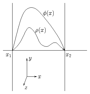
Figure 3.1: Electrostatic configuration independent of y and z with
conducting boundaries at x
1 and x
2 where ϕ = 0. This is a
second-order two-point boundary problem.
If we suppose (see Fig. 3.1) that the potential is held
equal to zero at two planes, x1 and x2, by placing
grounded conductors there, then its variation between
them depends upon the distribution of the charge density
ρ(x). Solving for ϕ(x) is a two-point problem. In effect,
this is a conservation equation for electric flux, E. Its
divergence is equal to the source density, which is
the charge density.
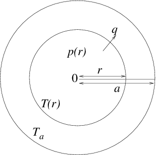
Figure 3.2: Heat balance equation in cylindrical geometry leads to a
two-point problem with conditions consisting of fixed temperature
at the edge, r=a and zero gradient at the center r=0.
In steady state, the total heat flux across the
surface at radius r (per unit rod length) must equal the total
heating within it:
|
2πr q = −2 πr κ(r) |
d T
dr
|
= | ⌠
⌡
|
r
0
|
p(r′) 2πr′dr′. |
| (3.4) |
Differentiating this equation we obtain:
|
|
d
dr
|
| ⎛
⎝
|
rκ |
d T
dr
| ⎞
⎠
|
= −r p(r). |
| (3.5) |
This second-order differential equation requires two boundary
conditions. One is T(a)=Ta, but the other is less immediately
obvious. It is that the solution must be
nonsingular at r=0, which requires that the
derivative of T be zero there:
3.2 Shooting
3.2.1 Solving two-point problems by initial-value iteration
One approach to computing the solution to two-point problems is to use
the same technique used to solve initial value problems. We
treat x1 as if it were the starting point of an initial value
problem. We choose enough boundary conditions there to specify the
entire solution. For a second-order equation such as (3.2) or
(3.5), we would need to choose two conditions: y(x1)=y1,
and dy/dx|x1=s, say, where y1 and s are the chosen
values. Only one of these is actually the boundary condition to be
applied at the initial point, x1. We'll suppose it is y1. The
other, s, is an arbitrary guess at the start of our solution
procedure.
Given these initial conditions, we can solve for y over the entire
range x1 ≤ x ≤ x2. When we have done so for this case, we
can find the value y at x2 (or its derivative if the original
boundary conditions there required it). Generally, this first solution will
not satisfy the actual two-point boundary condition at x2,
which we'll take as y=y2. That's because our guess of s was not
correct.
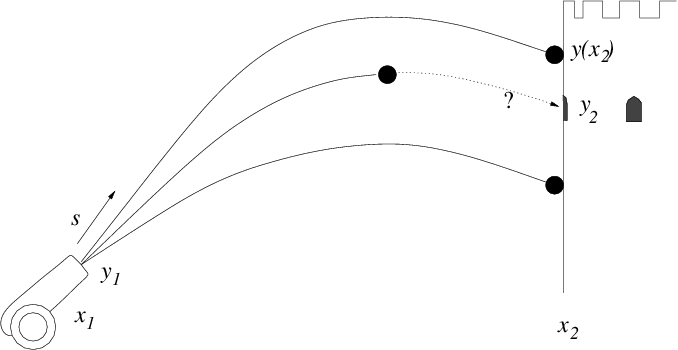
Figure 3.3: Multiple successive shots from a cannon can take advantage of
observations of where the earlier ones hit, in order to iterate the aiming
elevation s until they strike the target.
3.2.2 Bisection
Suppose we have a continuous
function f(s) over some interval [sl,su] (i.e. sl ≤ s ≤ su), and we wish to find a solution to f(s)=0 within that range.
If f(sl) and f(su) have opposite signs, then we know that
there is a solution (a "root" of the equation) somewhere between sl
and su. For definiteness in our description, we'll take f(sl) ≤ 0 and f(su) ≥ 0. To get a better estimate of where f=0 is, we
can bisect the interval and examine the value of f at the point
s=(sl+su)/2. If f(s) < 0, then we know that a solution must be in
the half interval [s,su], whereas if f(s) > 0, then a solution must
be in the other interval [sl,s]. We choose whichever half-interval
the solution lies in, and update one or other end of our interval to
be the new s-value. In other words, we set either sl=s or su=s
respectively. The new interval [sl,su] is half the length of the
original, so it gives us a better estimate of where the solution value
is.
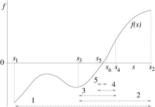
Figure 3.4: Bisection successively divides in two an interval in which there
is a root, always retaining the subinterval in which a root
lies.
3.3 Direct Solution
The shooting method, while sometimes useful for situations where
adaptive
step-length is
a major benefit, is rather a back-handed way of solving two-point
problems. It is very often better to solve the problem by constructing
a finite difference system to represent the differential equation
including its boundary conditions, and then solve that system
directly.
3.3.1 Second-order finite differences
First let's consider
how one ought to represent a second-order derivative as finite
differences. Suppose we have a uniformly spaced grid (or
mesh) of values of the independent variable
xn such that xn+1−xn=∆x. The natural definition of the
first derivative is
|
|
dy
dx
| ⎢
⎢
|
n+1/2
|
= |
∆y
∆x
|
= |
yn+1 − yn
xn+1 − xn
|
; |
| (3.7) |
and this should be regarded as an estimate of the value at the
midpoint xn+1/2=(xn+xn+1)/2, which we denote via a
half-integral index n+1/2. The second
derivative
is the derivative of the derivative. Its most
natural definition, therefore is
|
|
d2y
dx2
| ⎢
⎢
|
n
|
= |
∆(dy/dx)
∆x
|
= |
(dy/dx|n+1/2−dy/ dx|n−1/2)
xn+1/2−xn−1/2
|
, |
| (3.8) |
as illustrated in Fig. 3.5.
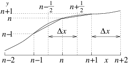
Figure 3.5: Discrete second derivative at n is the difference between
the discrete derivatives at n+
1/
2 and n−
1/
2. In a
uniform mesh, it is
divided by the same ∆x.
|
|
d2y
dx2
| ⎢
⎢
|
n
|
= |
(yn+1−yn)/∆x − (yn−yn−1)/∆x
∆x
|
= |
yn+1 − 2 yn + yn−1
∆x2
|
. |
| (3.9) |
Now think of the entire mesh stretching from n=1 to n=N. The
values yn at all the nodes can be considered to be a column vector
of length N. The second derivative can then be considered to be a
matrix operating on that column vector, to give the values of
eq. (3.9). So, written in matrix form we have:
|
| ⎛
⎜
⎜
⎜
⎜
⎜
⎜
⎝
|
|
| ⎞
⎟
⎟
⎟
⎟
⎟
⎟
⎠
|
= |
1
∆x2
|
| ⎛
⎜
⎜
⎜
⎜
⎜
⎜
⎝
|
|
| ⎞
⎟
⎟
⎟
⎟
⎟
⎟
⎠
|
| ⎛
⎜
⎜
⎜
⎜
⎜
⎜
⎝
|
| ⎞
⎟
⎟
⎟
⎟
⎟
⎟
⎠
|
, |
| (3.10) |
where the square N×N matrix has diagonal elements equal to −2. On the
adjacent diagonals, sometimes called subdiagonals, (indices n,n+1 and
n,n−1) it has 1; and everywhere else it is zero. This overall form is
called tridiagonal.
If we are considering the equation
where g(x) is
some function (for example g=−ρ/ϵ0 for our electrostatic
example) then the equation is represented by putting the column vector
(d2y/dx2|n) equal to the column vector (gn)=(g(xn)).
3.3.2 Boundary Conditions
However,
in eq. (3.10), the top left and bottom right corners of the
derivative matrix have deliberately been left ambiguous, because
that's where the boundary conditions come into play. Assuming they are
on the boundaries, the quantities y1 and yN are determined not
by the differential equation and the function g, but by the boundary
values. We must adjust the first and last row of the matrix
accordingly to represent those boundary conditions. A convenient way
to do this when the conditions consist of specifying yL and yR
at the left and right-hand ends is to write the equation as:
|
| ⎛
⎜
⎜
⎜
⎜
⎜
⎜
⎜
⎜
⎜
⎝
|
|
| ⎞
⎟
⎟
⎟
⎟
⎟
⎟
⎟
⎟
⎟
⎠
|
| ⎛
⎜
⎜
⎜
⎜
⎜
⎜
⎜
⎜
⎜
⎝
|
| ⎞
⎟
⎟
⎟
⎟
⎟
⎟
⎟
⎟
⎟
⎠
|
= | ⎛
⎜
⎜
⎜
⎜
⎜
⎜
⎜
⎜
⎜
⎝
|
| ⎞
⎟
⎟
⎟
⎟
⎟
⎟
⎟
⎟
⎟
⎠
|
. |
| (3.12) |
Notice that the first and last rows of the matrix have been made
purely diagonal, and the column vector on the right hand side (call it
h) uses for the first and last rows the boundary values, and
for the others the elements of g∆x2. These adjustments
enforce that the first and last values of y are always the boundary
values yL and yR.18
Once we have constructed this matrix form of the differential
equation, which we can write:
it is obvious that we can solve it by simply inverting the matrix
D and finding
(Or we can use some other appropriate matrix equation solution technique.)
In general, we must make the first and last rows of the matrix
equation into discrete expressions of the boundary conditions there.
If instead of Dirichlet boundary conditions (value is specified),
we are given Neumann conditions, that is, the derivative (e.g. dy/dx|1) is specified, a different adjustment of the
corners is necessary. The most obvious thing to do is to make the
first row of the matrix equation proportional to
|
(−1 1 0 ...) (y) = y2−y1 = ∆x(dy/dx|1). |
| (3.15) |
However, this choice does not calculate the derivative at the right
place. The expression (y2−y1)/∆x is the derivative at
x3/2 rather than x1, which is the boundary19. So the scheme (3.15) is not properly
centered and will give only first
order accuracy.20 A better
extrapolation of the derivative to the boundary is to write instead
for the first row
|
| ⎛
⎝
|
− |
3
2
|
2 − |
1
2
|
0 ... | ⎞
⎠
|
(y) = − |
1
2
|
(y3−y2)+ |
3
2
|
(y2−y1) = ∆x(dy/dx|1). |
| (3.16) |
This is a discrete form of the expression y′1 ≈ y′3/2−y"2.1/2∆x, which is accurate to second-order,
because it cancels out the first-order error in the derivative.
The same treatment applies to a Neumann condition at xN (but of
course using the mirror image of the row given in eq. (3.16)).
If the boundary condition is of a more general form (the
so-called Robin condition)
Then we want the first row to represent this equation discretely. The
natural way to do this, based upon our previous forms, is to make it
|
| ⎡
⎣
|
A | ⎛
⎝
|
1 0 0 ...)+ |
B
∆x
|
(− |
3
2
|
2 − |
1
2
|
0 ... | ⎞
⎠
| ⎤
⎦
|
(y) = −C. |
| (3.18) |
In addition to combining the previous inhomogeneous boundary forms,
this expression can also represent the specification of homogeneous
boundary conditions, or in other words logarithmic gradient
conditions. When C=0, the boundary condition is d(lny )/dx=y′/y=−A/B.
This form (with A/B=1) is the condition that one might apply to the
potential due to a spherically symmetric electrostatic charge at the
outer boundary, for example.
It may be preferable in some cases to scale the first row of the
matrix equation to make the diagonal entry the same as all the other
diagonals, namely −2. This is done by multiplying all the row's
elements of D, and the corresponding entry of h by a
factor −2/D11, or −2/DNN respectively. This can improve the
conditioning of the
matrix, making inversion easier and more accurate.
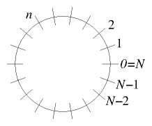
Figure 3.6: Periodic boundary conditions apply when the independent
variable is, for example, distance around a periodic domain.
|
| ⎛
⎜
⎜
⎜
⎜
⎜
⎜
⎜
⎜
⎜
⎝
|
|
| ⎞
⎟
⎟
⎟
⎟
⎟
⎟
⎟
⎟
⎟
⎠
|
| ⎛
⎜
⎜
⎜
⎜
⎜
⎜
⎜
⎜
⎜
⎝
|
| ⎞
⎟
⎟
⎟
⎟
⎟
⎟
⎟
⎟
⎟
⎠
|
= | ⎛
⎜
⎜
⎜
⎜
⎜
⎜
⎜
⎜
⎜
⎝
|
| ⎞
⎟
⎟
⎟
⎟
⎟
⎟
⎟
⎟
⎟
⎠
|
, |
| (3.19) |
which maintains the pattern 1,−2,1 for every row, without exception.
For the first and last rows, the subdiagonal 1 element that would be
outside the matrix, is wrapped round to the other end of the row. It
gives a new entry in the top right and bottom left
corners.21
3.4 Conservative Differences, Finite Volumes
In our cylindrical fuel rod example, we had what one might call a
"weighted derivative": something more complicated than a
Laplacian. One might be tempted to write it in the following way:
|
|
d
dr
|
| ⎛
⎝
|
rκ |
d T
dr
| ⎞
⎠
|
= rκ |
d2T
dr2
|
+ |
d(rκ)
dr
|
|
d T
dr
|
, |
| (3.20) |
and then use the discrete forms for the first and second derivative in
this expression. The problem with that approach is that first
derivatives are at half-mesh-points (n+1/2 etc.), while second
derivatives are at whole mesh points (n). So it is not clear how
best to express this multiple term formula discretely in a consistent
manner. In particular, if one adopts an asymmetric form, such as
writing dT/dr|n ≈ (Tn+1− Tn)/∆x, (just ignoring the
fact that this is really centered at n+1/2, not n), then the
error will be of second-order in ∆x. The scheme will be
accurate only to first-order. That's bad.
We must avoid that error. But even so, there are various different ways
to produce schemes that are second-order accurate. Generally the best
way is to recall that the differential form arose as a
conservation equation. It was the conservation of energy that
required the heat flux through a particular radius cylinder 2πrκdT/dr to vary with radius only so as to account for the power
density at radius r. It is therefore best to develop the
second-order differential in this way. First we form dT/dr in the
usual discrete form at n−1/2 and n+1/2. Then we multiply those
values by rκ at the same half-mesh positions n−1/2 and
n+1/2. Then we take the difference of those two fluxes writing:
|
|
| |
= | ⎛
⎝
|
rn+1/2κn+1/2 |
Tn+1−Tn
∆r
|
− rn−1/2κn−1/2 |
Tn−Tn−1
∆ r
| ⎞
⎠
|
|
1
∆r
|
|
|
| | |
| |
−(rn+1/2κn+1/2+rn−1/2κn−1/2) |
| |
| | |
|
|
| (3.21) |
The big advantage of this expression is that it exactly conserves the
heat flux. This property can be seen by considering
the exact heat conservation in integral form over
the cell consisting of the range rn−1/2 < r < rn+1/2:
|
2πrn+1/2κn+1/2 |
dT
dr
| ⎢
⎢
|
n+1/2
|
− 2πrn−1/2κn−1/2 |
dT
dr
| ⎢
⎢
|
n−1/2
|
=− | ⌠
⌡
|
rn+1/2
rn−1/2
|
p 2πr′dr′. |
| (3.22) |
Then adding together the versions of this equation for two adjacent
positions n=k,k+1, the
terms
cancel, provided the expression for
is the same at the
same n value regardless of which adjacent cell (k or k+1) it
arises from. This symmetry is present when using
|
dT
dr
| ⎢
⎢
|
n+1/2
|
=(Tn+1−Tn)/∆r
|
and the half-mesh
values of rκ. The sum of the
equations is therefore the exact total conservation for the region
rk−1/2 < r < rk+3/2, consisting of the sum of the two adjacent
cells. This process can then be extended over the whole domain,
proving total heat conservation. Approaching the discrete equations in
this way is sometimes called the method of "finite
volumes"22. The finite volume
in our illustrative case is the annular region between rn−1/2 and
rn+1/2.
A less satisfactory alternative which remains second-order accurate
might be to evaluate the right hand side of eq. (3.20) using
double distance derivatives that are centered at the n mesh as
follows
|
|
| |
= | ⎛
⎝
|
rnκn |
Tn+1−2Tn+Tn−1
∆r2
|
+ |
rn+1κn+1−rn−1κn−1
2∆ r
|
|
Tn+1−Tn−1
2∆r
| ⎞
⎠
|
|
|
| |
= |
1
∆r2
|
[ (rn+1κn+1/4+rnκn−rn−1κn−1/4) |
| |
| | |
| |
+(−rn+1κn+1/4+rnκn+rn−1κn−1/4) |
| |
|
|
| (3.23) |
None of the coefficients of the Ts in this expression is the same as
in eq. (3.21) unless rκ is independent of
position. This is true even in the case where rκ is known only
at whole mesh points so the half-point values in (3.21) are
obtained by interpolation. Expression (3.23) does not exactly
conserve heat flux, which is an important weakness. Expression
(3.21) is usually to be preferred.
Worked Example: Formulating radial differences
Formulate a matrix scheme to solve by finite-differences the equation
|
|
d
dr
|
| ⎛
⎝
|
r |
d y
dr
| ⎞
⎠
|
+ rg(r)=0 |
| (3.24) |
with given g and two-point boundary conditions dy/dr=0 at r=0
and y=0 at r=N∆, on an r-grid of uniform spacing ∆.
We write down the finite difference equation at a
generic position:
| |
dy
dr
| ⎢
⎢
|
n+1/2
|
= |
yn+1−yn
∆
|
.
|
Substituting this into the differential equation, we get
| |
−rngn= |
d
dr
|
| ⎛
⎝
|
r |
dy
dr
| ⎞
⎠
|
n
|
|
|
|
|
| ⎛
⎝
|
rn+1/2 |
dy
dr
| ⎢
⎢
|
n+1/2
|
− rn−1/2 |
dy
dr
| ⎢
⎢
|
n−1/2
| ⎞
⎠
|
|
1
∆
|
|
| |
| |
|
|
| ⎛
⎝
|
rn+1/2 |
yn+1−yn
∆
|
− rn−1/2 |
yn−yn−1
∆
| ⎞
⎠
|
|
1
∆
|
|
| |
| |
|
| (rn+1/2yn+1−2rnyn+rn−1/2yn−1) |
1
∆2
|
. |
| | (3.25) |
|
It is convenient (and improves matrix conditioning) to divide this
equation through by rn/∆2, so that the nth equation reads
|
| ⎛
⎝
|
rn+1/2
rn
| ⎞
⎠
|
yn+1−2yn+ | ⎛
⎝
|
rn−1/2
rn
| ⎞
⎠
|
yn−1 = −∆2gn |
| (3.26) |
For definiteness we will take the position of the nth grid point to
be rn=n∆, so n runs from 0 to N. Then the coefficients become
|
|
rn±1/2
rn
|
= |
n±1/2
n
|
=1± |
1
2n
|
. |
| (3.27) |
The boundary condition at n=N is yN=0. At n=0 we want
dy/dr=0, but we need to use an expression that is centered at n=0,
not n=1/2, to give second-order accuracy. Therefore following eq. (3.16) we write the equation at n=0
|
∆dy/dx|0=− |
1
2
|
(y2−y1)+ |
3
2
|
(y1−y0) = | ⎛
⎝
|
− |
3
2
|
2 − |
1
2
|
0 ... | ⎞
⎠
|
(y) = 0. |
| (3.28) |
Gathering all our equations into a matrix we have:
|
| ⎛
⎜
⎜
⎜
⎜
⎜
⎜
⎜
⎜
⎜
⎜
⎜
⎜
⎜
⎜
⎝
|
|
| ⎞
⎟
⎟
⎟
⎟
⎟
⎟
⎟
⎟
⎟
⎟
⎟
⎟
⎟
⎟
⎠
|
| ⎛
⎜
⎜
⎜
⎜
⎜
⎜
⎜
⎜
⎜
⎝
|
| ⎞
⎟
⎟
⎟
⎟
⎟
⎟
⎟
⎟
⎟
⎠
|
=−∆2 | ⎛
⎜
⎜
⎜
⎜
⎜
⎜
⎜
⎜
⎜
⎝
|
| ⎞
⎟
⎟
⎟
⎟
⎟
⎟
⎟
⎟
⎟
⎠
|
|
| (3.29) |
Fig. 3.7 shows the solution of an illustrative case.
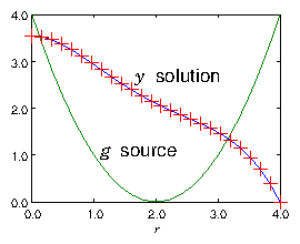
Figure 3.7: Example of the result of a finite difference solution for
y of eq. (
3.24) using a matrix of the form of
eq. (
3.29). The source g is purely
illustrative, and is plotted in the figure. The boundary points at
the ends of the range of solution are r=0, and r=N∆ = 4. A
grid size N=25 is used.
Exercise 3. Solving 2-point ODEs.
1.
Write a code to solve, using matrix inversion, a 2-point ODE of the form
on the x-domain [0,1], spanned by an equally spaced mesh of
N nodes, with Dirichlet boundary conditions y(0)=y0, y(1)=y1.
When you have got it working, obtain your personal expressions for
f(x), N, y0, and y1 from
http://silas.psfc.mit.edu/22.15/giveassign3.cgi. (Or use
f(x) = a + bx, a = 0.15346,
b = 0.56614,
N = 44,
y0 = 0.53488,
y1 = 0.71957.) And solve the
differential equation so posed. Plot the solution.
Submit the following as your solution:
- Your code in a computer format that is capable of being
executed.
- The expressions of your problem f(x), N, y0, and y1
- The numeric values of your solution yj.
- Your plot.
- Brief commentary ( < 300 words) on what problems you faced and how you solved them.
2.
Save your code and make a copy with a new name. Edit the new code so
that it solves the ODE
on the same domain and with the same boundary conditions, but with the
extra parameter k2. Verify that your new code works correctly for
small values of k2, yielding results close to those of the previous
problem.
Investigate what happens to the solution in the vicinity of k=π.
Describe what the cause of any interesting behavior is.
Submit the following as your solution:
- Your code in a computer format that is capable of being
executed.
- The expressions of your problem f(x), N, y0, and y1
- Brief description ( < 300 words) of the results of your
investigation and your explanation.
- Back up the explanation with plots if you like.