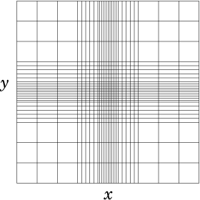
 (a)
(a)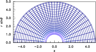 (b)
(b)
| HEAD | PREVIOUS |
| (4.1) |
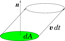
| dtv. |
^
n
| dA = dt v.dA |
| (4.2) |
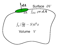 Using Gauss's (divergence) theorem, illustrated
in Fig. 4.2, that for any
vector field u (here u=ρv), the integral over
a closed volume of the divergence is equal to the surface integral of
the vector:
Using Gauss's (divergence) theorem, illustrated
in Fig. 4.2, that for any
vector field u (here u=ρv), the integral over
a closed volume of the divergence is equal to the surface integral of
the vector:
| (4.3) |
| (4.4) |
| (4.5) |
|
∂
| =0 |
| (4.6) |
| (4.7) |
| (4.8) |
| (4.9) |
|
| (4.11) |
| (4.12) |
| (4.13) |
| (4.14) |
| (4.15) |
| (4.16) |
| (4.17) |
| (4.18) |
| (4.19) |
| (4.20) |
| (4.21) |
|
| (4.23) |
| (4.24) |
| (4.25) |
|
∂ψ
| =0 |
| (4.26) |
|
|
| (4.29) |
| p2 |
∂2 ψ
| + q2 |
∂2 ψ
| =0 |
| p2 |
∂2 ψ
| − q2 |
∂2 ψ
| = ψ |
|
∂2 ψ
| + 4 |
∂2 ψ
| + |
∂2 ψ
| =0 |
|
∂2 ψ
| + 2 |
∂2 ψ
| + |
∂2 ψ
| =0 |
|
∂2 ψ
| + p |
∂ψ
| = ψ |
|
∂2 ψ
| + |
∂2 ψ
| + |
∂2 ψ
| =0 |
| p |
∂ψ
| + qy |
∂ψ
| = 1 |
| L = |
∂2
| +2 |
∂2
|
| HEAD | NEXT |